NVGate Formula Computation

Description of NVGate Computation: This document describes the different computations that are done inside the analyzer.

Computation of overall Level

Frequently asked question : Why the overall RMS level of my Spectrum mismatches with the sum of spectrum lines ?

ENBW is the key... :)

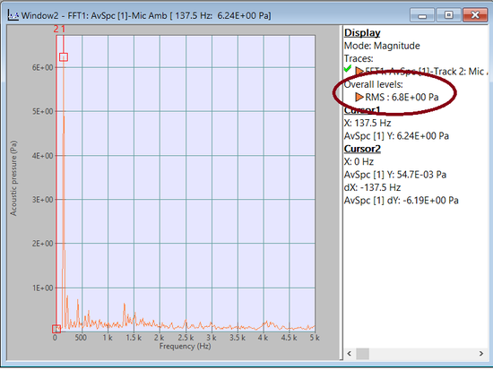
On NVGate you can find the RMS overall level on several windows. For exemple, on FFT spectrum it can be found here:

If you want to recompute this value using the FFT spectrum line you need to do the following computation:

First you have to sum the amplitude of the frequency line between the freq min and the freq max A(f). (be careful if you have RMS value you have to put each amplitude to square before sum it. (A(f)² ). Then you have to devide that by the ENBW of the ponderation windows (for information it’s 1.5 for haning windows.) then do the square root of this sum.

That is to say:

Ap (f) = A(f)²/ENBW

Then you sum S (f1, f2) = sum from f1 to f2 of Ap(f).

Then you have to put the square root of this sum to have the overall power : P(f1,f2) ) = SQRT (S (f1, f2))

How to find ENBW coefficent ?

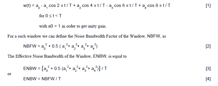
You will find it on weighting windows page. To sum up:

ENBW rectangular windows = 1

ENBW hanning windows = 1.5

ENBW hamming windows = 1.36

ENBW kaiser bessel windows = 1.8

ENBW Flat Top windows = 3.77

---

Computation of FFT

For each record of signal with duration of T , the corresponding Fourier Transform is computed as:

Analysis Windows

Weighting windows are defined in the OROS analyzer as follows:

Computation of Spectra in Spectral Averaging

Computation of Spectra in Time Averaging

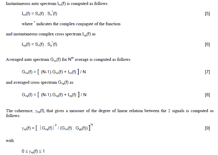
Instantaneous auto spectrum and instantaneous cross spectrum are computed as follows for spectral averaging.

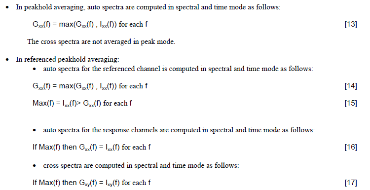
Linear, Exponential, Peakhold and Referenced Peakhold Averaging

If user has selected M averages, the successive averages are computed as follows:

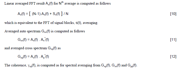
• In linear mode, the equations [7], [8] in spectral mode or [10] in time mode are used to compute successive averages from the 1^st one to the M^th and then the analyzer stops. In these equations N varies respectively from 1 to M.

• In exponential mode, the M first averages are computed as in linear mode and then the analyzer continues averaging with N equal to M.

Time Integration or Derivation of Spectra

Auto and cross spectra can be modified in order to get the same effect as a single or double integration or derivation in time domain.

Scaling of Auto and Cross Spectra

Basically auto spectra and cross spectra are internally scaled in EU² relative to a pure sine signal (EU stands for Engineering Unit, which is the physical unit of the analyzed signal).

For example, if user injects an 1 EU rms pure sine at a frequency exactly equal to one of the FFT lines, the corresponding line for I_xx, I_xy, G_xx and G_xy is equal to 1 EU².

Display of Auto and Cross Spectra

Auto spectrum and cross-spectrum module can be displayed relatively to Amplitude or Power Spectrum Density.

When Amplitude is selected the spectrum line values are displayed relatively to a pure sine signal. For example, if user injects a 1 EU rms pure sine at a frequency exactly equal to one of the FFT lines, the displayed values are:

1.000 EU rms in RMS mode,

1.414 EU peak in PEAK mode,

2.828 EU pp in PEAK to PEAK mode

The selection of one of these modes is available in the Input setup dialog box for each channel.

Computation of frequency band power

Computation of auto-correlation and cross-correlation

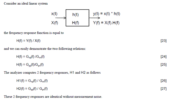
Frequency Response Measurement

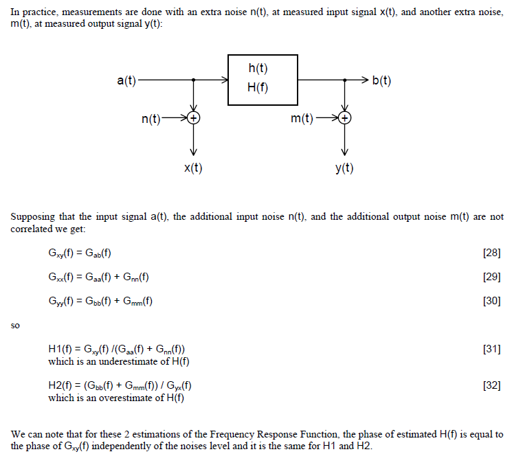
From two auto spectra and the associated cross spectrum, the analyzer can compute the frequency response of a linear system. Two cases are considered for result interpretation, without or with extra measurement noises.

Without measurement noise

With measurement noise:

Real and Imaginary parts:

Interpolation of Peaks in Spectra

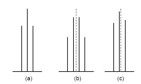
When analyzing a sinusoid using FFT, this one appears as a peak in the spectrum.

As the spectrum is only measured at discrete frequencies, so we generally get an error in both amplitude and frequency of the associated highest line in the spectrum, for example:

(a) sinusoid frequency equal to a spectrum line

(b) sinusoid frequency at the middle of two spectrum lines

(c) sinusoid frequency near a spectrum line

These errors are compensated by an interpolation technique using the window filter characteristics of the weighting function:

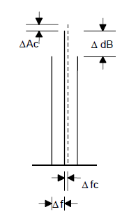
Knowing the characteristics of the analysis window, the difference ΔdB, between the two highest spectrum lines gives the correction ΔAc (amplitude) and Δfc (frequency) to be applied in order to get the exact values of sinusoid amplitude and frequency.

In the OROS analyzer, the frequency correction is computed, at user request, with a resolution equal to 1/32^th of the analysis resolution Δf.

Cepstrum

The Module Cepstrum display is available in the FFT analysis with option "diag".

Where F_xx is the power spectrum of the time signal f_x(t)

τ is the "quefrency" (this variable has the dimension of time)

Cepstrum analysis can be used as a tool for the detection of periodicity in a spectrum, for example families of harmonics with uniform spacing.

A high "quefrency" represents rapid fluctuations in the spectrum (small frequency spacings) and a low "quefrency" represents slow changes with quefrency (large frequency spacings). Note that the quefrency does not give information on the absolute frequency but only about frequency spacings.

Measurement scalar Level