Difference between revisions of "Sound Quality Lite"
| Line 544: | Line 544: | ||
Sharpness is compute according to Zwicker DIN 45692 method. | Sharpness is compute according to Zwicker DIN 45692 method. | ||
[[File:zwicker.png|400px]] | |||
===Roughness=== | ===Roughness=== | ||
Revision as of 11:43, 20 August 2024
Installation
Download
Download Last Version of Sound Quality Lite V1.2.
Equipment required for the installation
USB drive containing OROS Sound Quality LIte software installation setup "SoundQualityLiteSetup.msi".
NVGate software must have been installed first.
Installation of NVGate software
First you need to install NVGate.
Installation of Sound Quality Lite software
Run the “SoundQualityLiteSetup.msi” program, and the following window is displayed:

Click on “Next”, and the following window is displayed:

Read the terms of the license agreement and select "I accept the terms in the license agreement" if you agree. Click on “Next”, and the following window is displayed:

Select the installation directory. It is highly recommended to keep the default location: C:\OROS\Programs\Sound Quality Lite. Click on “Next”, the following window is displayed:

Click on “Install”, and wait until the following window is displayed:

Click on “Finish” to exit the setup wizard, and OROS Sound Quality Lite software is successfully installed.
NOTE: Before launching the software, please plug OROS USB dongle if your license is dongle locked, or connect the PC to the analyzer and launch NVGate in the connected mode if your license is instrument locked.
User Interface
Introduction
OROS Sound Quality Lite is a software providing:
- An auditory model optimized according to psychoacoustics results,
- An interactive filter set for designing and analyzing sound,
- And a tool for playback and comparison.
Click

To launch the software. The NVGate software is required to work and will be started automatically if not already running.
The following window is displayed when it is ready.

Sound Quality Lite main window
Project manager
On the left part, the Project Manager is shown. The project manager is synchronized with the NVGate project manager. Training samples are installed together with the software: 'Sound Quality Samples' and may be used when first using the software.

Project Manager
Main Page
On the right, the main functionalities are shown.
|
- Filter design and interactive filtering | |
|
- Sound playback | |
|
- Psycho-acoustic parameter calculation | |
Click on each button to active the responding page.
'Recent Filters' and 'Recent Playlists' will also be shown below.

Sound Quality Lite start page
Menu
- File
- Create, open and save Filters
- Exit the module.

File menu
- View
- Elements
- Switch among different pages

View menu
- Option
- Settings for filter folder and audio device
- Language

Language settings

Settigs dialog box
- Help
- Tutorial for the SoundQuality module
Hereafter the functionalities will be introduced step by step.
Psychoacoustics Parameters Calculation
The Psychoacoustics module calculates Articulation Index (AI), Loudness (LO), Sharpness (SH), Roughness (RO), Fluctuation strength (FL), Tonality (TO) and out of the sound signal.
Psychoacoustics results selection
Step 1: Add sound track into Track List
At the lower part of the window, there is 'Projects' and 'Tracks' page.
- 'Projects' shows the projects in NVGate Projects folder.
- 'Tracks' lists all pre-selected sound channel, and provide a clearer way to access to the signal to be analyzed.
Right click on the project or sound sample to be analyzed, and click 'Add to Track List' to add to 'Tracks'.

Once there are new measurements in NVGate, it is necessary to 'Refresh' accordingly in the 'Projects'.
Step 2: Analyze Sounds
On the 'Start Page', Click on 'Analyze Sound(s)' button to turn to 'SoundAnalysis' page.

Step 3: Choosing the psychoacoustics parameters to be analyzed
Drag and drop signals from 'Tracks' to the right window to do the analysis.
Click on the checkboxes to select or deselect PSY parameters to be calculated.

Psychoacoustics metrix selection
By clicking on the checkbox in front of the signal name, all the parameters will be selected.
By clicking on the checkbox on top of the parameter, all the signals will be selected.
Step 4: Modify analysis parameters
Press
to change parameters for AI and Loudness.

AI and Loudness parameters selection
Step 5: Calculate and review results
Press 'Calculate' button to do the calculation. Results will be saved as a measurement and can be viewed in NVGate. Name of the measurement is in the format SQResult and numbers.

Saving psychoacoustics results
In the measurement, all calculated results are included.

Psychoacoustics results in the project manager
User may Drag&Drop these results to see the curve or number.

Psychoacoustics results profiles display

Psychoacoustics results vumeters display
Filtering
The interactive filtering is used for filter design, interactive filtering and playback with online filters.
Step 1: Filter setup
The Filter Explorer (FE) is a powerful tool that lets you design various IIR filter types (low pass - LP, high pass - HP, band pass - BP, band stop - BS, equalizer - EQ and order equalizer - OEQ) using different design algorithms (first/second order filters, higher order Butterworth and Chebychev filters). All the parameters of the different kinds of filters are listed in the further chapter "Filter Design setup parameters".

Equalizer filter example
The design parameters can be specified either numerically or graphically using the mouse. Designed filters can be saved to a file and loaded afterwards and may then be redesigned.
The Filter Explorer allows you to design, save and apply a cascade of up to 32 filters. In a cascade various filter types and filters of different orders can be mixed. Note that online filtering performance depends on the number of cascaded filters, the overall filter order and the computational power of your computer. Single filters can be added and removed from the cascade easily by checking the box.

Single (black curve) response and cascaded filters response (yellow curve)
Filters are designed by specifying their magnitude response. The Filter Explorer displays the magnitude response, the phase response or the group delay of a single filter (single filter curve) or of the filter cascade (full response curve in Yellow).

Contextual menu (right click) when designing a filter
Click on
to save the filter.
Step 2: Using filters
The effect of designed filters can be approved by online-filtering of a sound. The filter may be redesigned while online filtering.
- Play Control
 : Play
 : stop
 :loop
:loop- [[Image:SOUND_QUALITY_28.png]: use filter
 : delete track
 :use headset equalization

Play control toolbar
The selected track with darker background is the one to be filtered.
The colormap showed below is the filtered spectrogram. And it is changed simultaneously with the interactive filter set. Of course, when showing the colormap, the user can select proper filters. In the example below, the difference caused by applying different 'Filter 3' could be seen on the colormap.
|
|
|
| Example before changing filter 3 | Effect of changing filter 3 |


Filter design setup parameters
Filters can be set up in different ways. In the Sound Quality Lite Explorer:
Equalizer (EQ), low pass (LP), high pass (HP), band pass (BP), band stop (BSTP) filters and order equalization (OEQ) can be designed.
All filters are realized as digital IIR filters. All filters except equalizer filters (EQ & OEQ) are designed by transforming an analog prototype low pass into the digital domain. Butterworth and Chebyshev designs are available for higher order filters.
In the Filter Control Panel, design parameters can be selected independently for each filter type. All possible design parameter are listed in the table below.


Filter design setup parameters table
Graphical Filter Design
All design parameters can be set numerically or graphically by changing the coordinates of squares in the magnitude response display. The squares can be moved by placing the mouse arrow over the black square until it is highlighted blue. Then, the square which represents certain design parameters can be moved as long as the left mouse button is pressed.
Example
The graphical filter design is explained for a Chebyshev band pass filter with a center frequency of 8 kHz and one octave bandwidth (5657 Hz) and a prototype order of 5. The order of the digital filter is 10. The transition width between pass band and stop band is 1 kHz. The attenuation in the stop band is more than 30 dB. The ripples extent from 0 dB to -3 dB (+3dB attenuation). The center frequency of 8 kHz is the geometrical mean of the upper pass frequency (11314 Hz) and the lower pass frequency (5657 Hz).

Filter settings example
Defining the pass attenuation, the bandwidth and the upper pass frequency
The left upper square (square 1) and the right upper square (square 2) define the pass attenuation and the upper and lower pass frequency.
The vertical movement (pass attenuation) of square 1 and square 2 is coupled. The horizontal movement (lower and upper pass frequency) is coupled by the bandwidth relation. If the bandwidth depends on frequency, square 1 can not be moved horizontally. It will be moved automatically when square 2 is moved. If the bandwidth does not depend on frequency the center frequency is kept constant when square 1 is moved and the bandwidth is kept constant when square 2 is moved.
Defining the stop attenuation and the transition width
The left lower square (square 3) and the right lower square (square 4) define the minimum stop attenuation and the transition width. The vertical movement (minimum stop attenuation) of square 3 and 4 is coupled. The transition width is changed by horizontal movement of square 3 or square 4.
LP/HP – Low/High Pass Filter
Fixed order Filters
- Low/high pass filters are defined by a single point of the magnitude response (pass frequency, pass attenuation). If the pass attenuation is 3 dB the pass frequency is often called the cut-off frequency.
- For low pass filters the band below the pass frequency is the pass band and the band above the pass frequency the stop band. The maximum gain of 0 dB is at dc.
- For high pass filters the band above the pass frequency is the pass band and the band below the pass frequency the stop band. The maximum gain of 0 dB is at the nyquist rate.
Higher order Filters
Variable order low/high pass filters are defined by one point of the magnitude response (pass frequency, pass attenuation) and the prototype order.
FILTER DESIGN SETTINGS

|

|

| |
BP/BS– Band Pass/Stop Filter
Fixed order Filters
Band pass/stop filters are defined by two points of the magnitude response [(lower pass frequency, pass attenuation), (upper pass frequency, pass attenuation)]. The difference between upper and lower pass frequency is the bandwidth. The bandwidth is often defined as the frequency difference between the 3 dB attenuation points.
- For band pass filters the band in between the pass frequencies is the pass band. Frequencies below and above the pass band characterize the stop band. The maximum gain of 0 dB is at the center frequency in the pass band.
- For band stop filters the band between the pass frequencies is the stop band. Frequencies below and above the stop band characterize the pass band. The maximum gain of 0 dB is at dc and at the Nyquist rate.
Higher order Filters
Butterworth and Chebyshev (pass band ripple or stop band ripple) designs are available for higher order filters.
- The Butterworth low pass has a monotone magnitude response.
- Chebyshev filters have either ripples in the pass band or in the stop band. Due to the ripples Chebyshev filters have steeper magnitude characteristics than Butterworth filters with the same filter order.
In OROS Sound Quality Lite, either a first Butterworth order or higher order Butterworth and Chebyshev filters can be designed. For band bass/stop filters the digital filter order is two times the prototype order otherwise it is identical to the prototype order.
Band pass/stop filters are defined by two points of the magnitude response [(lower pass frequency, pass attenuation), (upper pass frequency, pass attenuation)] and the prototype order.
For Chebyshev filters with pass band ripples the pass attenuation is equal to the extent of the ripples in the pass band. The order is computed so that a minimum attenuation is achieved at one stop frequency for low/high pass filters and at the lower and the upper stop frequency for band pass/stop filters. Since only integer orders can be realized the stop attenuation of the digital filter is in general slighter better than specified. The frequency difference between pass and stop frequency is the transition width.
- For band pass filters the lower stop frequency is defined as one transition width below the lower pass frequency. The upper stop frequency is defined as one transition width above the upper pass frequency.
- For band stop filters the lower stop frequency is defined as one transition above the lower pass frequency. The upper stop frequency is defined as one transition width below the upper pass frequency.
Filter design settings

Bandwidth of Band Pass and Band Stop filters
The lower pass frequency (f_lower) is defined as the bandwidth subtracted from the upper pass frequency (f_upper). The bandwidth can be specified in several ways in the Filter Control Panel either directly or dependent on frequency and the bandwidth type. Available bandwidth types are Absolute, Octave, Bark and ERB. Except for the type Absolute an additional divider (fraction) can be specified. For example if the bandwidth type is Octave and fraction is 3 then the bandwidth is 1/3 Octave.

Bandwidth parameters

EQ – Equalizer Filter
Equalization filters are second order IIR filters. They are defined by 3 parameters (center frequency, center gain and quality factor). The forward and backward coefficients of these filters are obtained from these 3 parameters. Form function of an equalization filter with center frequency of 649 Hz, gain of 12.6 and quality factor of 2.

Equalizer filter settings
OEQ – Order Equalizer Filter
The order equalizer filter makes sense if a tach signal was recorded. In this case it requires to have been saved on the ext trigger channel.

Order equalizer filter settings
The definition of order equalization filters is identical to the definition of equalization filters except that the form function is order dependent (Order = frequency/RPM´60. Order equalization is valid only if a RPM function is linked to the sound file. If not, designing such a filter will have no effect on the sound file.
Playback
In the playback module, the user is able to setup a playlist to do comparison listening with or without saved filters.
Step 1: Playlist setup
Common way to add a sample to the playlist is
- Drag one track to 'Left' or 'Right' channel.
- Select a saved filter or not.
- Choose the reference tach.
- Input the time range.
- Click on 'Add' to add.
- Continue with other tracks.
Another way to proceed is to Drag & Drop sound samples from the track list to the 'Playlist' window.
- Basic information will be shown, such as Name, Location, Tach info and Range.
- 'Key' is automatically assigned to each sample. User can switch among these samples using number keys on the keyboard.

Playlist window
Step 2: Play and Listen
Drag & Drop sound samples from the track list to the 'Playlist' window.
Click on these buttons to
Playback toolbar
|
Play |
Use filter |
|
Stop |
Delete track |
|
Previous |
Use headset equalization |
|
Next |
Edit filter |
|
Loop |
Save and open playlist |
Toolbar icons
Filtering Orders
In order to filter out orders from a signal, one must use a signal with a tach recorded on the external trigger. Among the "Sound Quality Samples" installed with the version, there is one signal called "Runup with Tach": this signal can be used for order tracking filtering.
1. Create a filter with only 1X filtered. The 3X can be seen on the spectrogram

Filtering orders, step 1
2. Create a filter with 1X, 2X and 3X filtered. One see the 3X filtered.

Filtering orders, step 2
One should choose, a time range to be played and add it in the playlist as shown below:

Filtering orders, step 3
Listening to them sequentially through the playlist below, one can ear the difference and the effect of the 3X filtering.

Playlist dialog
Showing the tach profile:
By a right click in the graph area and choosing view "Tach", one can display the Tach profile

Tach profile
Psychoacoustics theoretical background
Loudness
The loudness analysis computes loudness versus time and specific loudness versus critical-band rate versus time pattern. Stationary signals are analyzed in accordance with DIN 45631 and ISO 532B. By including nonlinear post-masking algorithms, non-stationary signals can also be analyzed.
In order to calculate further psychoacoustical parameters like Roughness, data are stored with a time resolution of 2 ms.
Loudness computations should be used for all situations, where the human hearing system is the final receiver. E.g.: Two vacuum cleaners may have different loudness, although their A-weighted sound pressure level is the same.
The basic scheme for the loudness calculation according to Zwicker is as follows:
- For each time interval the sound levels in 20 approximated critical bands are computed using a third octave filter bank.
- The critical band levels are weighted according to the transfer from the sound field through the outer and middle ear.
- The weighted critical band levels are called excitation levels.
- The excitation levels are transformed to specific loudness (core loudness) values.
- The transform from excitation to specific loudness depends on the excitation at threshold in quite (ETHQ).
ETHQ depends on frequency for frequencies below 1 kHz and may be individually different for normal hearing and hearing-impaired persons.
The nonlinear post-masking algorithm is applied to the core loudness values.
After post-masking, frequency and level dependent (upward) spectral masking is modeled which results in 240 specific loudness values at the interval of 0.1 Bark.
By integrating the specific loudness, the loudness at this time interval is computed.
The only parameter for the basic loudness calculation is the type of sound field which can be Free or Diffuse.
The analysis time interval is fixed to 2ms.
The number of frames to be computed according to the chosen analysis time range is given in the dialog.
The following table summarizes the parameters of the loudness parameters dialog.
| Parameter | Description |
| Sound Field | The sound field parameter matches the calculation according to the recording conditions. It can be set to free or diffuse sound field conditions. Default: Free |
| Time interval | The time interval is fixed to 2 ms. This high temporal resolution corresponds to the temporal resolution of the human ear and is needed in order to calculate roughness out of specific loudness. |
| NISO532B | Compute stationary Loudness according to ISO532B |
Loudness parameters table

Loudness parameters dialog
Sharpness
Sharpness is computed by the integration of the weighted specific loudness values.
In order to incorporate temporal integration effects, loudness and sharpness are low pass filtered.
Sharpness is compute according to Zwicker DIN 45692 method.

Roughness
Spectral analysis of roughness and fluctuation strength yields additional data for time varying signals. Almost all technical signals show modulations and fluctuations produced by periodic or stochastic processes. Sharpness, loudness spectrum, roughness spectrum and fluctuation strength spectrum are the fundamental parameters for the calculation of annoyance or sound quality. The unit for roughness is Asper (1 Asper = 100 cA). The unit for fluctuation strength is Vacil (1 Vacil = 100 cV).
The Roughness Sequence Length defines the length of the (loudness) data window which is used to compute specific roughness and overall roughness for a point in time. The data windows overlap by a certain amount because the sequence length is always longer than the time interval. The most reliable results are obtained with a roughness sequence length of 500 ms. For short signals (< 2 s) a sequence length of 200 ms may be useful.

Fluctuation Strength
The Fluctuation Strength Sequence Length defines the length of the (loudness) data window which is used to compute specific fluctuation strength and overall fluctuation strength for a point in time. The data windows overlap by a certain amount because the sequence length is always longer than the time interval. The most reliable results are obtained with a fluctuation sequence length of 1000 ms. For short signals (< 4 s) a sequence length of 500 ms may be useful.

Tonality
OROS SQ Prominence Analysis gives objective measures on the prominence of tonal components in a sound. OROS SQ offers two different approaches to compute the prominence of tonal components:
The Tone-to-Noise Ratio (TNR) and the Prominence Ratio (PR).
The TNR is computed either according to ANSI S1.13-1995 or to the new draft of the E DIN 45681–2002.
The PR is computed according to ANSI S1.13-1995.
The TNR is defined as the ratio of the power of the tone to the power of the critical band centered on that tone (excluding the tone power).
Masking effects by components from outside the critical band are not taken into account.
A tone becomes just audible when its TNR exceeds the frequency dependent masking index av.
All measures are based on time averaged FFT power spectra using a Hanning window.
TNR method according to E DIN 45681-2002
The procedure according to E DIN 45681-2002 is based on a time averaged A-weighted FFT power spectrum.
The averaging time for stationary sounds must be at least 30 s.
The frequency resolution of the power spectrum may not exceed 4 Hz.
Tones are automatically identified at local maxima in the averaged spectrum above 100 Hz
where the level is at least 6 dB above the mean level of the surrounding critical band.
In general more than one spectral line with the following properties represent a tone:
|
|
|
|
|
|
The last two properties are called the clarity criterion, which is not required for non-stationary sounds.
The noise power in a critical band is computed by an iterative procedure that excludes all tonal components in the critical band. Critical bands are always centered on tones.
The powers of all tones within a critical band are added to the total tone power.
The TNR is the level difference of the total tone power to the noise power.
The measure DL is the difference of the TNR to the masking index (DL = TNR '''- 'av).
The maximum DL is taken as the result.
Negative DL's are set to a lower limit which depends on the tone frequency and the FFT frequency resolution.
The masking index depends on the frequency of the tone. It amounts to –2 dB around 200 Hz and decreases to –6 dB for frequencies up to 16 kHz.
| Frequency (Hz) | DL=TNR-av (dB) | av (dB) | TNR (dB) |
| 100 | -12,4 | -2,0 | -14,4 |
| 200 | -12,4 | -2,0 | -14,5 |
| 500 | -13,0 | -2,3 | -15,3 |
| 1000 | -14,4 | -2,8 | -17,2 |
| 2000 | -17,1 | -3,5 | -20,6 |
| 5000 | -21,9 | -4,5 | -26,4 |
| 10000 | -25,9 | -5,2 | -31,2 |
Masking Index a'v 'and lower limits for DL and TNR (FFT frequency resolution=3,9 Hz) according to E DIN 45681-2002.
If the tone frequencies in a sound vary slightly over time, the procedure must be applied for 12 time intervals of 10 s.
Then, the energetical mean of the maximum DL (mean DL) for each time interval is taken as the result.
In the case of intervals without tones, DL is set to the lower limit of a 1kHz tone before averaging.
A tone penalty between 0 and 6 dB is computed depending on mean DL and given in the text report window.
The maximum DL over all time intervals (max DL) is also computed.
In addition the power spectrum averaged over the whole analysis time range
and the maximum DL for that global spectrum (global DL) is computed.
If the time interval is equal to the analysis time range, then mean DL, max DL and global DL are all identical.
| DL = TNR - a'v '(dB) | Penalty (dB) |
| <= 0 | 0 |
| 0 < DL <= 2 | 1 |
| 2 < DL <= 4 | 2 |
| 4 < DL <= 6 | 3 |
| 6 < DL <= 9 | 4 |
| 9 < DL <= 12 | 5 |
| 12 < DL | 6 |
Penalty depending on DL according to E DIN 45681-2002.
TNR method ANSI S1.13 1995
The procedure according to ANSI S1.13 1995 is based on a time averaged unweighted FFT power spectrum.
A minimum of 25 independent power spectra over a time of at least 15 s must be averaged.
The separation of spectral lines belonging to a tone or to masking noise is not defined clearly in ANSI S1.13 1995.
Therefore the identification of tones in the spectrum as well as the computation of tone level is achieved using the E DIN 45681-2002 procedures.
If there is more than one tone within a critical band, the critical band is centered on the tone with the highest level (primary tone).
The power of the tone with the second highest level (secondary tone) is added to the total tone power if its frequency is close enough.
The noise power is the power in the critical band centered on the primary tone excluding the tone power
and the power of a secondary tone if it exists.
The TNR is the level difference of the total tone power to the noise power.
The maximum TNR for all tones in the power spectrum is taken as the result.
The masking index is not taken into account.
TNR's below -4 dB are set to the lower limit as defined in E DIN 45681-2002.
A tone is classified as prominent when its TNR exceeds 6 dB (10 dB above the average masking index of -4 dB).
If the tone frequencies vary slightly over time, the procedure may be applied at a certain time interval (not specified in ANSI S1.13 1995).
Then the energetical mean of the maximum TNR for each time interval (mean TNR) is computed.
In the case of intervals without detected tones, TNR is set to the lower limit of a 1kHz tone as defined in E DIN 45681-2002 before averaging.
The maximum TNR for all time intervals (max TNR) is computed.
In addition the power spectrum averaged over the whole analysis time range
and the maximum TNR for that global spectrum (global TNR) is computed.
The global TNR is the result according to ANSI S1.13 1995.
If the time interval is equal to the analysis time range then mean TNR, max TNR and global TNR are all identical.
AI (Articulation index)
Intelligibility is for voice communications, the capability of being understood - the quality of language that is comprehensible. Intelligibility has several meanings: clearness, explicitness, lucidity, comprehensibility, perspicuity, legibility, plain speaking, etc.
One of the earliest attempts to measure by machine the intelligibility of a speech transmission system, the Articulation Index was developed by Bell Telephone Laboratories in the 1940's.
AI is based on the idea that the response of a speech communication system can be divided into twenty frequency bands, each of which carries an independent contribution to the intelligibility of the system, and that the total contribution of all the bands is the sum of the contributions of the individual bands. (AI may also be measured using one-third octave or octave bands.) Signal-to-noise ratios are computed for each individual band, then weighted and combined to yield an intelligibility score.
The AI (ANSI S3.5-1969) varies in value from 0 (completely unintelligible) to 1 (perfect intelligibility). An AI of 0.3 or below is considered unsatisfactory, 0.3 to 0.5 satisfactory, 0.5 to 0.7 good, and greater than 0.7 very good to excellent. Apart from the ANSI standard, other definitions of the AI exist, such as Unikeller used in the automotive industry, NVH and more. The differences are the weighting and speech levels used in each third octave bands.
OROS SQ enables to compute the Articulation Index according to 3 methods: the ANSI S3.5-1969, the unikeller and the NVH. Both are based on the calculation of the third octave spectrum of the signal (from the band 200 Hz to the band 6300 Hz) and a comparison with a third octave reference speech spectrum. The difference spectrum is then weighted by a set of coefficients depending on the method chosen. The generic form of the calculation is :
AI = W * (Vref + A – V) / N
W is the spectrum of weighting coefficients, Vref is the speech reference spectrum, V is the signal spectrum.
For NVH, A = 30 et N = 30.
The Text Report window gives detailed information on the Prominence Analysis computation parameters and results.
For each analysis time interval the results for up to 10 detected tones with the highest TNR and PR measures are reported.
The highest measures for each analysis time interval are the ones shown in the graphs PR vs.Time and TNR vs.Time.
The next figure shows the computation parameters and the results for the first analysis time interval (Frame 1):
In the computation parameters the realized FFT frequency resolution can be found.
The Prominence Analysis results for the first time interval are shown.
More than 10 tones were detected in frame 1.
FAQ about loundness
When we compute the loudness in Sound Quality Lite we get the above list of results in NVGate.
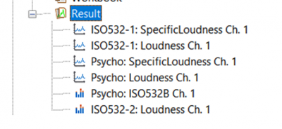

Let’s find below the explanation of this loudness
• ISO532-1 Specific loudness ch 1
According to the standards ISO532-1 : It is computed on the whole signal, it computed a loudness value in every 2 ms.
• ISO532-1: Loudness ch1 According to the standards ISO532-1 : the spectrum is computed on the whole signal. The standards is for stationary signal.
• Psycho: Specific Loudness ch1” and “Psycho:loudness ch 1 Not standardize loudness, but based on DIN 45631/A1-2010. (One value every 2 ms for profile, and compute on the whole signal for the spectrum)
• Psycho IS0 532 B: According to IS0 532 B. It is computed on the whole signal, the standard is used for stationary signal, so there is only one value.
• ISO532-2: Loudness Ch1: ISO532-2 standard : It is the “American Loudness standard” (This standard replaces ISO 532 A (loudness according to Stevens) and it is based on ANSI S3.4-2007 standard for calculating stationary loudness according to Moore. It is computed on the whole signal, the standard is used for stationary signal, so there is only one value.
Short history about loudness:
There is 2 main ways to compute the loudness
- The “European” way : Zwicker method
ISO 532-1 (release in 2017 ) this standards is a revision and based on ISO 532 B. It is based on DIN 45631/A1 standard for determining both stationary and time variable noise according to Zwicker.
The new standards ISO 532-1 add:
- avoid any uncertainty regarding the practical implementation. - Better continuity and comparability than earlier calculations.
- The “Amercian” Way.
ISO 532-2 this standards is based and replaced ISO 532 A (loudness according to Stevens).
The standard is based on the American ANSI S3.4-2007 standard for calculating stationary loudness according to Moore and Glasberg.