Modal Signal Processing

Signal processing

Signal processing wizard is designed to set the parameters for signal processing. Many signal estimations can be realized, such as power spectrum estimation, multiple input multiple output frequency response function estimation, and coherence function estimation, and so on. Five steps should be performed in this wizard: Estimation, Detrending, Decimation, Fast Fourier Transform (FFT)], and Windowing.

Estimation

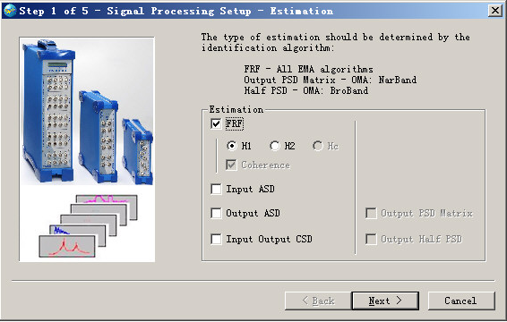
Various signal estimation process can be set in this page. You must estimate the ’FRF’ if you want to perform modal parameters identification in the case of EMA. H1,H2 and Hc are three different methods for FRF estimation. Reference signal is needed for Hc method. You must estimate the ’Output PSD Matrix’(for OMA NarBand Full) or ’Output half PSD’(for OMA BroBand, OMA NarBand Half, and so on) if you want to perform modal parameters identification in the case of OMA.

The next step of signal processing wizard is Detrending.

Detrending

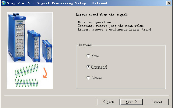
The purpose of detrending is to condition the time domain signals, remove their constant or linear trend.

The previous step of signal processing wizard is Estimation, and the next step is Decimation.

Decimation

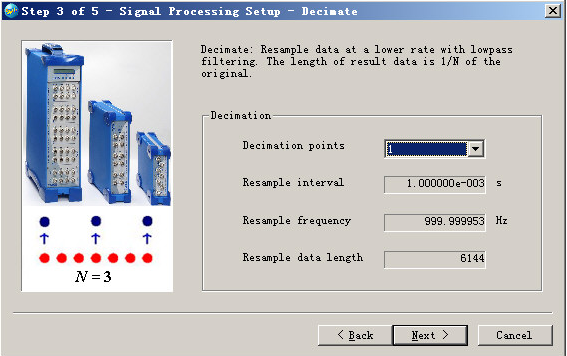
The purpose of decimation is to reduce the range of analysis frequency. For example, you are interest in the frequency range of 0~10 Hz, and the sampling frequency is 256 Hz, then you should set the decimation points to 10.

The basic principle of decimation is reserve part of points and removing the others: if the decimation points is N, the length of data will be 1/N of original data. To prevent the estimation from frequency aliasing, a low-pass filter is necessary in this process.

There are not any anti-aliasing filters in some low-cost data acquisition. It will greatly improve the quality of estimation for you to sample data with high frequency and then decimate them in Modal, partly compensating for the loss of anti-aliasing filters.

The previous step of signal processing wizard is Detrending, and the next step is setup of FFT].

Setup of FTT

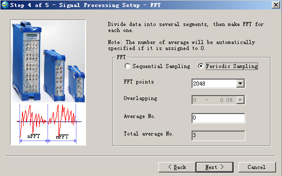
In this page, parameters for fast Fourier transform (FFT) will be set to transfer the time domain signals to frequency domain.

’Sequential Sampling’ means that the data was sampled sequentially, without any pause. A typical instance is to sample data sequentially under random excitation. "Periodic Sampling’ means that the data in the file was sampled periodically. A typical instance is to sample multiple frames of data in a hammer impact test, for the sake of performing average in the spectrum estimation. The practical significance of "Periodic Sampling" is the overlap percent is set to zero in FFT.

’FFT Points’ specifies the length of each segment in the transform. The optional list will be confirmed by the software according to the length of imported data automatically. You can select one from this list. When the data points has less than ’FFT points’, zeros will be padded, and truncated if it has more.

’Overlapping’ specifies the percent of overlap between each segment. The purpose of overlap is to increase the times of average. For an example of 2048 data length and 1024 FFT points, if the overlap percent is set to 0, the original data can be divided into two segments for FFT (the first segment is from 1 to 1024, and the second part is from 1025 to 2048); When the overlap percent is set to 50%, the number of overlap points is 512, and the original data can be divided into three segments (the first segment is from 1 to 1024, and the second segment is from 513 to 1536, and the third segment is from 1025 to 2048).

’Average No.’ specifies the number of average during the FFT calculation. Its default value is 0, which means the maximum possible average numbers. When the number specified by the user is larger than the maximum average number, it will be modified to the maximum average number automatically

The previous step of signal processing wizard is decimation, and the next step is windowing.

Windowing

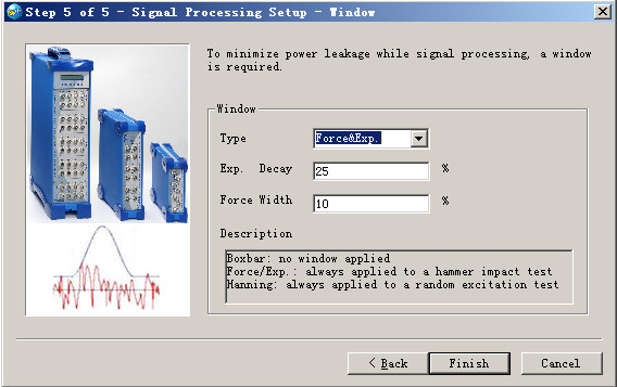
You can specify the windowing functions for the FFT in this page. The truncation and non-periodicity of signal will cause energy leakage and lead to alias error in the frequency domain. The main purpose of windowing is adding time weight functions to the signal to filter the non-periodicity part and reduce leakage. Six kind of window function such as Boxcar, Exponential, Force & Exponential, Hanning, Hamming, Flattop is provided and can be employed for different cases.

Boxcar

Boxcar window, called as Transient window also, has the shape of rectangle. It adds the same weight to all parts of the time history, i.e. no weight is added.

The Boxcar function has a value of 1 over its length and it only truncation the signal simply. It can be applied to the signal such as periodic (period random) and transient (Chirp, Burst Chirp) signal generally.

Exponential

The shape of the exponential window is that of a decaying exponential. By assigning the time const, the exponential window damps the signal, ensuring that the signal fully decays by the end of the sample block.

Exponential function can be applied commonly to the measurement of light damping system.

The following equation defines the exponential window:

W(t)=e^-βt

Where β is a constant. In Modal, Td is defined as the exponential decay time over which exponential window function decays from 1 to 1/e, in this case , β=1/ Td. When applying exponential function to a signal, damping of the system will be increased and should be modified. The damping ratios and frequencies can be automatically modified in Modal if the exponential window is applied by the signal processing wizard. When the input data is FRFs which were estimated by applying exponential window, you should remember to specify the decay time (with unit of ms) in the configuration file.

Note: The value you should fill in this interface is not β, but the percentage of β constitutes to the sampling period.

Force & Exponential

In a force window, the front part of the signal is preserved and the others are set to 0. The time length of the preserved signal is named force width. When Force & Exponential window is selected, exponential window is applied to both channels while force window is only applied to the reference channel.

Force window is very useful for the hammer impact test and it can wipe off the fluctuation of the force signal and greatly improve SNR (Signal Noise Ratio).

Note: You should fill the percentage of these values constitute to the sampling period as well.

Hanning

Hanning window is also named random window and has a shape similar to that of half a cycle of a cosine wave. It decays the start and end part of the signal and enforce the signal to become periodic.

It is a general-purpose window and its typically applied to the test excited by random noise.

Hamming

Hamming window is similar to Hanning window and it can further decrease the side lobe.

Flattop

Namely cosine window, the flattop has the flatness power shape and the higher amplitude accuracy while poor frequency resolution.

The flattop window is most useful in accurately measuring the amplitude of specified frequency components such as filter characters.

This is the last step of the signal processing wizard, and the previous step is setup of FFT. Press the ’Finish’ button to confirm all the parameters set in the wizard, and you can begin to signal processing now.

The sampling times can be set to 2.56 or 2. Usually in an EMA analysis it is set to 2.56, and in an OMA analysis it is set to 2. If the sampling times is 2.56, then the number of the spectral line will be 1/2.56 of the FFT length, and the analysis frequency range will be 1/2.56 of the sampling frequency. If the sampling times is 2, then the number of the spectral line will be half of the FFT length, and the analysis frequency range will be half of the sampling frequency.

After signal processing, the result data will be displayed under the directory of ’Data\Setup?\Estimate" in the ’Data’ page of workspace short pane, such as FRF (frequency response function), COH (coherence function), Pxx (input auto power spectral density function), Pyy (output auto power spectral density function), Pxy (input and output cross power spectral density function), OPSD (output power spectral density matrix) and HPSD (half power spectral density function). Double click these items, and relevant curves or lists will be displayed in the main window.

If you want to do signal processing with other parameters, please run the wizard and process again. Before the new signal processing, all the result got from last signal processing will be refreshed or deleted automatically.