Difference between revisions of "Modal practical"
| Line 1: | Line 1: | ||
==GEOMETRY BUILDING== | |||
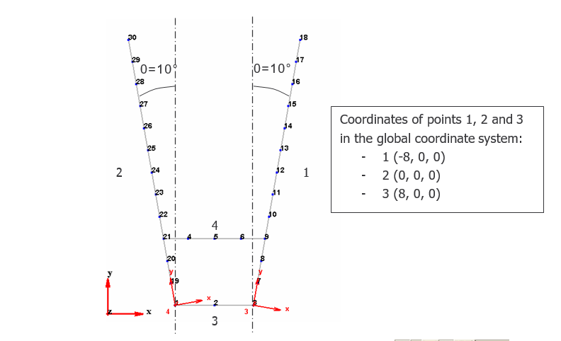
<font color="#363639">The goal of this part is to model the cantilever by the geometry below. The different steps of the procedure are described here. | <font color="#363639">The goal of this part is to model the cantilever by the geometry below. The different steps of the procedure are described here. | ||
Revision as of 14:41, 16 July 2020
GEOMETRY BUILDING
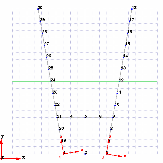
The goal of this part is to model the cantilever by the geometry below. The different steps of the procedure are described here.
|
- Line 1
Click on `add line’
in the geometry toolbar. A line is defined as follow:
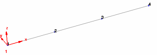
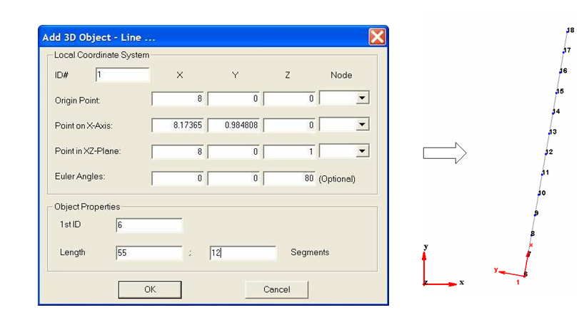
For each line, the software associates a Cartesian coordinates system. The line is defined by the origin of this system, the direction of X axis, the length and the number of segments.
To create the line 1, enter the following parameters:
Note: for the local coordinate system parameters, enter parameters about origin point and Euler angles only.
Rename the point 6 in point 3 by opening `Config review’ and make the modification in the
`nodes’ window.
==Note: When the `config review’ is activated, click on `modeling interface’ button
to display both `geometry’ and `config review’ windows.==
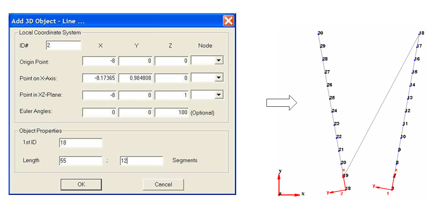
- Line 2
Click on `add line’
and enter the following parameters
Remove the line between point 18 and 19 by clicking on `select lines’ in the toolbar Select the line 18-19 and delete it.
Rename the point 18 in point 1.
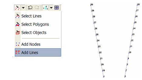
Create the lines 1-19 and 3-7 by clicking on
`add lines’ in the toolbar
and link the points directly on the geometry. (left click on the 2 points and right click to end the operation)
- Line 3
Click on `add lines’
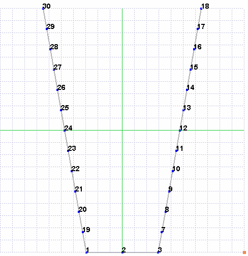
and link point 1 and 3
To create point 2, click on `add nodes’
, a grid is displayed to help you to position new points. Right click to fix a new point and rename it in point 2.
- Line 4
Create the points 4, 5 and 6 with the grid and add lines to link them.
- Experimental coordinates systems
Regarding the axis definition for the acquisition, 2 local coordinates systems should be added respectively on the nodes of line 1 and 2.
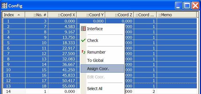
In the `config review’ select the nodes of lines 1. Right click and select `Assign Coord.’
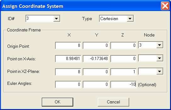
To reproduce the experimental conditions, enter the following parameters
In the `Config review’ select the nodes of line 2. Right click and select `Assign Coord.’ Enter the following parameters
Delete the coordinates systems 1 and 2 in `config review’ /coordinates
Results
|
|
For this demo, use the data file `CANTILEVER HAMMER DATA.uff’ containing the Frequency Response Functions acquired with one impact hammer and 2 accelerometers.
In the File menu, click on Import/Data files (UFF). The following window is displayed.
Select `acceleration’ for response type,
`Frequency domain’ for data type.
Click on the button
, select the file `CANTILEVER HAMMER DATA.uff’ and click on OK.
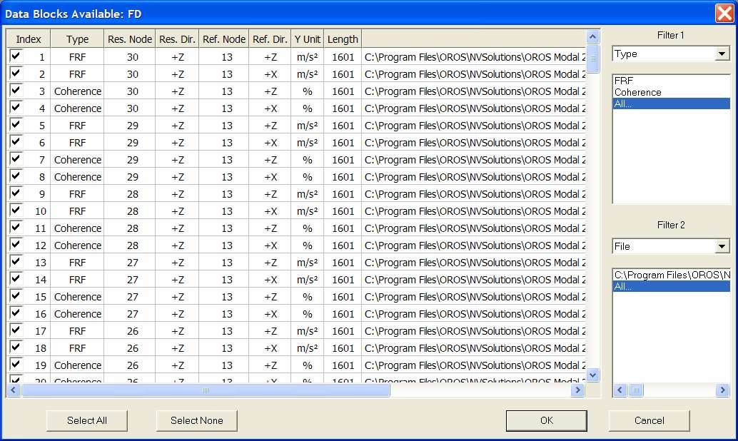
The following window shows all the results contained in the imported file with their characteristics. Information of nodes and directions can be modified if an error occurs.
Any filters are available to import a part of the data only.
Here all the data will be used, so click on OK. The FRFs are directly displayed in the software.
All the FRFs can be visualized.
|
By using the Control Panel (Series select), all the FRFs can be displayed. For each result, there is information about the DOFs (node, direction).
Several types of displayed are available by right clicking on the graph: magnitude/phase, real/imaginary, Nyquist.
By right clicking on the graph and selecting `Showed Series…’, you can display several FRFs on the same graph for comparison.
|
|
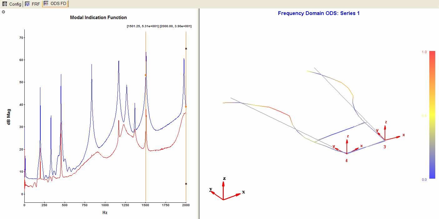
In the operation tree, double click on `ODS: Freq Domain The following interface is displayed.
On the left, the Modal Indication Function (MIF) shows the modes in the frequency band. Position the cursor on the peaks and visualize the corresponding mode shapes on the right.
What is the MIF?
MIF can be employed in not only EMA, but also OMA. In EMA case, the number of MIFs equals the number of excitations or references. In OMA case, the number of MIFs equals the minimum number of responses of each setup. The MIFs consist of the singular values of frequency response function matrix (FRF), output power spectral density matrix (OPSD), or half power spectral density matrix (HPSD).
By the powerful singular value decomposition, the real signal space is separated from the noise space. Therefore, the MIFs exhibit the modes effectively. A peak in the MIFs plot usually indicate the existence of a structural mode, and two peaks at a same frequency point means the existence of two repeated modes. Moreover, the magnitude of the MIFs always implies the strength of a mode.
Two separated modes
Weak modes
Two pairs of repeated modes
Sometimes we should note the cross modes. For example, in the below figure, the peak in the second MIF curve doesn’t indicate a mode. It’s formed by the cross of two modes.
|
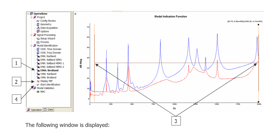
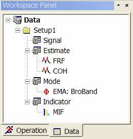
In the operation tree:
- select EMA Broband (A red icon appears near the method),
- the MIF is displayed,
- Select a large frequency band by positioning the cursors and double click to fix them (a black line between the 2 cursors appears),
- click on start identification
- Preliminary determination of the number of modes in the selected frequency band according to the MIF plot, and fill it in the edit box of "Preset Modes No." Then the BroBand software will calculate a default "minimum order" according to this number. The relationship between "Preset Modes No." and "Minimum Order" is: minimum order = (preset modes No)*Ni/2, where Ni means the number of input. Change the number of "Order Span" if necessary. The BroBand software will estimate the poles with a range of system order from "Minimum Order" to "Maximum Order", where Maximum order= Minimum order + Order Span-1. The default order span is 12.
- Modal identification
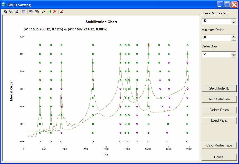
Press the button of "Start Modal ID" to obtain frequency stability diagram. This operation might take a little longer time to finish a complex structure with large number of modes and measurement coordinates. In the stability diagram, a shape symbol represents one pole. A pole in this diagram may represent a physical (i.e. structural) mode or a spurious (or noise) mode. It is normally not difficult to distinguish physical/structural) mode from spurious/noise mode by the distribution of poles. Generally speaking, a physical/structural mode can be identified in each proper number of order, while for a spurious/noise pole it usually is not the case. There are five kinds of symbols to indicate the poles:
| Symbol | Description |
| o | The pole is not stable. (The poles obtained from the first order are always considered as unstable.) |
| f | The frequency of the pole does not change within the tolerance of 1%. |
| v | The frequency of the pole does not change within the tolerance of 1%, and the pole vector does not change within the tolerance of 10% |
| d | The frequency of the pole does not change within the tolerance of 1%, and the damping of the pole does not change within the tolerance of 10%. |
| s | Both frequency, damping and vector are stable within the tolerances: the frequency of the pole does not change within the tolerance of 1%; the pole vector does not change within the tolerance of 10%; and the damping of the pole does not change within the tolerance of 10%. |
- Auto selection of structural modes
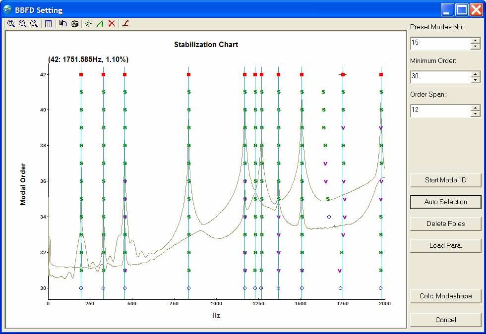
Press the button of "Auto Selection" or
, the OM2 selects the physical/structural modes automatically. While move the mouse cursor on a pole, the modal frequency and damping ratio corresponding to this pole will be shown. You can move the mouse on
different poles to check the stability via small change of the modal frequency and/or damping ratio.
==
Note: Manual selection of structural modes: a pole can also be manually selected by clicking it or deselected it by same operation. A selected pole will be marked with a shape symbol==
- Mode shapes calculation
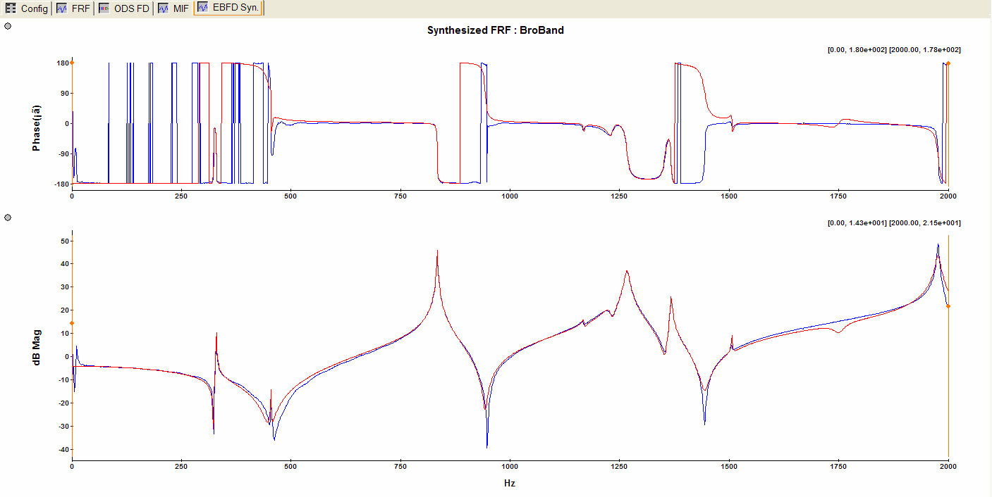
Press the button of "Calc. Modeshape" to confirm the pole section and BroBand software start to estimate the mode shapes and to calculate the synthesized FRFs.
- Results visualization
To visualize the list of the modes, double click on `EMA: BroBand The list of results will be displayed. By right clicking on a mode and selecting `animate’, the corresponding mode shape will be showed.
|
The first way to check the results is to look at the coherence between the experimental FRFs and the synthesized ones in the selected frequency band.
To go further, results from 2 different methods can be compared using the Modal Assurance Criterion (MAC).
Here, we have results from Broadband method. The repertory `Cantilever modal demo’ contains a file `MIMO1 results’ with the modal parameters obtained from MIMO1 method.
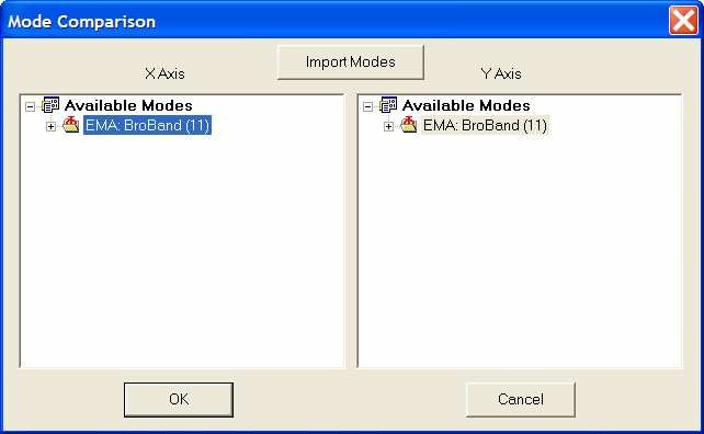
| In the operation tree, double click on MAC |
The following window is displayed |
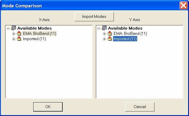
Click on Import Modes and select the file `MIMO1 results’ and OK
|
The project can be saved in a workspace containing data, geometry, results… It’s also possible to save independently each part of a project.
- The data (FRFs) are saved in uff 58
- Create a file uff 15 containing the geometry by clicking on File/export/geometry,
- Export the modal results by right clicking on the modes list and select `Export Modes…’
- Create a file .avi with a mose shape by displaying a mode shape and click on
in the control panel.
