Difference between revisions of "Balancing single/dual plane"
| (84 intermediate revisions by 2 users not shown) | |||
| Line 3: | Line 3: | ||
==Introduction== | ==Introduction== | ||
A rotor is a shaft rotating around its axis during service. In general such a rotor consists of a shaft with one or more discs fitted to the axle. Such discs can be fly wheels, grinding wheels, turbine wheels, etc. The shaft is usually running in bearings allowing the rotation of the body. Depending on their rotational speed, two basic categories can be defined to classify rotors: <u>rotors with rigid shaft</u>, and <u>rotors with flexible shaft</u>. <br> | A rotor is a shaft rotating around its axis during service. In general, such a rotor consists of a shaft with one or more discs fitted to the axle. Such discs can be fly wheels, grinding wheels, turbine wheels, etc. The shaft is usually running in bearings allowing the rotation of the body. Depending on their rotational speed, two basic categories can be defined to classify rotors: <u>rotors with rigid shaft</u>, and <u>rotors with flexible shaft</u>. <br> | ||
<br> | <br> | ||
If the operating speed remains below half of the first critical bending speed, the shaft does not deflect : it may be considered as a rotor with a rigid shaft. At such operational speeds and due to the non circular cross section of the rotor, the axis of rotation (Z) and the inertial axis (Δ) does not coincide (e.g. the mass is not evenly dispatched in a section of the shaft). This may results in a tumbling movement of the structure, | If the operating speed remains below half of the first critical bending speed, the shaft does not deflect : it may be considered as a rotor with a rigid shaft. At such operational speeds and due to the non circular cross section of the rotor, the axis of rotation (Z) and the inertial axis (Δ) does not coincide (e.g. the mass is not evenly dispatched in a section of the shaft). This may results in a tumbling movement of the structure, this amplitude depends on the bearing clearance and stiffness. In any case, the bearings are subjected to unnecessary or even not allowed loads. | ||
[[Image:Unbalanced_shaft_schem.png|framed|center|''Unbalance : | [[Image:Unbalanced_shaft_schem.png|framed|center|''Unbalance : Inertial axis does not coincide with rotational axis.<br> The unevenly mass distribution is represented by "m"'']]<br> | ||
At higher speeds the shaft will deflect, due to is own stiffness. In that case, it might be considered as a rotor with flexible shaft. Depending on the position of the discs on the shaft they can even be inclined and thus create an oil whirl. In that case, the Multiplane Balancing solution must be used.<br> | At higher speeds the shaft will deflect, due to is own stiffness. In that case, it might be considered as a rotor with flexible shaft. Depending on the position of the discs on the shaft they can even be inclined and thus create an oil whirl. In that case, the Multiplane Balancing solution must be used.<br> | ||
| Line 80: | Line 80: | ||
'''Accelerometer''' | '''Accelerometer''' | ||
The measurement direction of the accelerometer must be referred to the tach sensor position. This can be done by the "Angular correction" in the analyzer setup. In our example in '''Sketch 1,''' the '''angular correction''' </font>is '''90°''' and the <font color="#339966">'''offset''' </font>is -'''15 °'''. | The measurement direction of the accelerometer must be referred to the tach sensor position. This can be done by the "Angular correction" in the analyzer setup. In our example, in '''Sketch 1,''' the '''angular correction''' </font>is '''90°''' and the <font color="#339966">'''offset''' </font>is -'''15 °'''. | ||
'''Tip''' | '''Tip''' | ||
| Line 120: | Line 120: | ||
===Physical Background=== | ===Physical Background=== | ||
The <u>initial run</u> | The <u>initial run</u> analyzes the behavior of the rotor due to its initial unbalance. | ||
During the <u>test run</u>, the applied test masses modify the position of the unbalance. This yields the sensitivity of the rotor. Thus with the knowledge of the reaction of the rotor to added masses, suitable masses can be calculated to compensate the initial unbalance. | During the <u>test run</u>, the applied test masses modify the position of the unbalance. This yields the sensitivity of the rotor. Thus with the knowledge of the reaction of the rotor to added masses, suitable masses can be calculated to compensate the initial unbalance. | ||
For <u>balancing in one plane</u>, just one test mass and one test run is necessary. It is important that the angular position of the initial unbalance is changed | For <u>balancing in one plane</u>, just one test mass and one test run is necessary. It is important that the angular position of the initial unbalance is changed significantly by the test mass. Take this into account when choosing test weight and position. | ||
When <u>balancing in two planes</u>, two test runs are necessary. For each run only one test mass is necessary positioned in one of both planes respectively. Again in both test runs the position of the unbalance must be changed by the test masses. | When <u>balancing in two planes</u>, two test runs are necessary. For each run only one test mass is necessary to be positioned in one of both planes respectively. Again, in both test runs the position of the unbalance must be changed by the test masses. | ||
'''Assumptions''' | '''Assumptions''' | ||
| Line 134: | Line 134: | ||
'''Example''' | '''Example''' | ||
Imagine a rotating machine to be balanced when standing untightened on the floor. After the test mass is mounted the increased unbalance | Imagine a rotating machine to be balanced when standing untightened on the floor. After the test mass is mounted the increased unbalance causes the machine to move. Holding or fixing the machine during the test run will cause wrong balancing results. To overcome this you must choose a lower test mass or position to reduce the unbalance. If this doesn<nowiki>'</nowiki>t work you could fix the machine during the <u>complete</u> balancing procedure. After this basic balancing, execute a second complete balancing procedure with the machine unfixed (in normal operating conditions). | ||
'''General advice''' | '''General advice''' | ||
| Line 187: | Line 187: | ||
==Settings== | ==Settings== | ||
Settings follow the same steps whether it is for one plane balancing (single) or two planes balancing (dual). Thus, description below is given for the two planes | Settings follow the same steps whether it is for one plane balancing (single) or two planes balancing (dual). Thus, description below is given for the balancing of a two planes rotor. | ||
====Project management==== | ====Project management==== | ||
=====Project Manager window===== | |||
===== | |||
{|border="2" cellspacing="0" cellpadding="4" width="100%" | {|border="2" cellspacing="0" cellpadding="4" width="100%" | ||
|'''(1)''' | |'''(1) Project Base : '''List of the project in the current Project Base<br>'''(2) Projects Base Path :'''Change the Project Base<br>'''(3) Project Browse : ''' Add project in the current Base. | ||
|'''(4)''' | |'''(4) New Project :''' Create a new project<br>'''(5) Exit :''' Exit the balancing program | ||
|} | |} | ||
[[Image: | [[Image:Bal_Proj_Manager.png|framed|none]] | ||
=====Load an existing Project===== | |||
To load an existing project, select the project in the '''(1) Project Base''' and click OK. | |||
You can import a project form another database by clicking on '''(3) Browse Project'''. | |||
=====Create a new Project===== | =====Create a new Project===== | ||
To create a new project, click on '''(4) New Project''' and enter the name of the project in the appearing ribbon at the bottom of the window : | |||
[[Image:New_Proj.png|framed|none]]<br> | |||
'''( | |||
The new project will then appear in the Project Base, select it and click OK : | |||
[[Image: | [[Image:New_Proj2.png|framed|none]]<br> | ||
====Select the configuration of the machine==== | ====Select the configuration of the machine==== | ||
| Line 261: | Line 236: | ||
To choose your transducer from the transducer data base, click on '''Transducer'''. | To choose your transducer from the transducer data base, click on '''Transducer'''. | ||
''' | ====Transducer database==== | ||
[[Image:Balancing_22.png|framed|none]] | |||
''Transducer data base'' | |||
For easier and faster adjustment use the transducer data base. | |||
Input your transducer in the list shown by clicking the corresponding fields and adjust an input transducer label, unit and sensitivity. | |||
To select a transducer click in the corresponding line, and choose the analyzer channel, where this transducer is connected to. Click '''Set.''' | |||
The transducer data base can be saved and reloaded. | |||
It is also possible to create several data bases for example for different users and their transducers. | |||
====Setting the tachometer==== | |||
To set the tachometer, you need to go into the "Speed" tab : | |||
[[Image:Bal_Tacho.png|framed|none]] | |||
'''Note: '''Your tach signal must have one pulse per revolution. If you have more than one pulse, you can set the maximal speed as Real_speed*Pulse/rev. | |||
* Set the range, coupling and slope for this tach signal. | * Set the range, coupling and slope for this tach signal. | ||
* Input the balancing speed. | * Input the balancing speed. | ||
* Set the number of averages for your measurements. | * Set the number of averages for your measurements. | ||
====Set a phase adjustment==== | |||
To set a phase adjustment, you can specify the position of the sensors. To enter the menu, click on "Position": | |||
[[Image:Bal_Position.png|framed|none]]<br> | |||
The position of each sensors and the tachometer can be set : | |||
[[Image:Bal_Position_Menu.png|framed|none]]<br> | |||
'''Note :''' The 0° position is the position of the tachometer reflector on the shaft. The angle are counted positive in the anti-rotation direction. | |||
====Saving the channel and measuring setup==== | |||
If you want to make sure | All setup settings can be saved and reloaded with "<u>S</u>ave" and "<u>L</u>oad" buttons.<br> | ||
'''Note:''' '''The balancing module''' always starts with the last analyzer settings used.<br> | |||
You do not need to do all adjustments for a new project. Just load the setup of an existing project.<br> | |||
'''Tip:'''<br> | |||
If you want to make sure you always start with the same settings, create a reference project with all settings adjusted properly. Each part of the project is saved with a specific extension. | |||
* Reference Project = *.WSR | * Reference Project = *.WSR | ||
| Line 293: | Line 295: | ||
For a new Project with these Settings: Load Reference Project. | For a new Project with these Settings: Load Reference Project. | ||
This is now the last project that has been used | This is now the last project that has been used: | ||
* Create New Project: It has the settings of the Reference Project. | * Create New Project: It has the settings of the Reference Project. | ||
| Line 301: | Line 303: | ||
* Click "Continue" to proceed to the next step. | * Click "Continue" to proceed to the next step. | ||
---- | ---- | ||
====Rotor geometry and balancing quality==== | ====Rotor geometry and balancing quality==== | ||
{|border="2" cellspacing="0" cellpadding="4" width="100%" | {|border="2" cellspacing="0" cellpadding="4" width="100%" | ||
|'''(1)''' No. of mass positions | |'''(1)''' No. of mass positions both planes<br>'''(2)''' Radius for both planes<nowiki>[</nowiki>mm<nowiki>]</nowiki> <br>''' (3)''' Offset of the first mass position regarding the reference at 0° <nowiki>[</nowiki>Deg<nowiki>]</nowiki><br>'''(4)''' Click on Apply to display the circle<br>'''(5)''' Unit of Unbalance <nowiki>[</nowiki>g mm<nowiki>]</nowiki>, <nowiki>[</nowiki>oz in<nowiki>]</nowiki> or <nowiki>[</nowiki>g in<nowiki>]</nowiki> | ||
|'''(6)''' Rotor mass<br>'''(7)''' Speed RPM<br>'''(8)''' Quality class<br>'''(9)''' | |'''(6)''' Rotor mass<br>'''(7)''' Speed RPM<br>'''(8)''' Quality class (def. in ISO1940/1)<br>'''(9)''' Maximal residual unbalance (according to ISO1940) <nowiki>[</nowiki>g mm<nowiki>]</nowiki><br>'''(10)''' Residual unbalance <nowiki>[</nowiki>oz in<nowiki>]</nowiki> | ||
|} | |} | ||
[[Image: | [[Image:Bal_Rotor_Quality.png|framed|none]] | ||
''Rotor geometry and balancing quality'' | ''Rotor geometry and balancing quality'' | ||
In this window, the test runs and plane are positioned as follow : | |||
[[Image:Bal_2_Test_Prep.png|framed|none]]<br> | |||
You can export and reload a configuration with the "Export" and "Load" buttons. | |||
==One plane balancing== | ==One plane balancing== | ||
| Line 373: | Line 336: | ||
If you use accelerometers for your measurement the signal can be integrated to show vibration velocity. | If you use accelerometers for your measurement the signal can be integrated to show vibration velocity. | ||
'''The analyzer is now ready for measurement.''' | The '''Rotor''' window is automatically displayed. You can now prepare your test run or close this window to set it up later: | ||
Your settings are shown by a red point in the polar graph. | |||
There are three methods: | |||
* '''Remove test masses ''' : The test mass will be removed after test for example bolts etc. | |||
* '''Keep test masses ''' : The test mass cannot be removed after the test (for example for welding or drilling etc…) | |||
* '''Displace two masses per plane '''for machines with slidable balancing weights. | |||
The figure below shows an example where test mass is to be removed. The test mass of 4.2 grams is set at position 4 (105°; radius 100 mm). | |||
The settings are saved automatically when closing the window. To use these settings in another project, click on export '''(1)''' </font>and save it in the sub directory of the other project. Proper settings can be loaded from another project '''(2)'''</font>. | |||
[[Image:Bal_1_Test_Prep.png|framed|none]] | |||
Click on OK to come back on the measurment window.<br> | |||
'''The analyzer is now ready for measurement.'''<br> | |||
To start the analyzer click '''(1)''' or <nowiki>[</nowiki>F2<nowiki>]</nowiki> and the Measurement is displayed. | To start the analyzer click '''(1)''' or <nowiki>[</nowiki>F2<nowiki>]</nowiki> and the Measurement is displayed. | ||
| Line 387: | Line 367: | ||
'''(d)''' Balancing calculation | '''(d)''' Balancing calculation | ||
[[Image: | [[Image:Bal_Wind.png|framed|none]] | ||
* ''Measurement display - start analyzer'' | * ''Measurement display - start analyzer'' | ||
====Measurement monitor settings==== | |||
[[Image:Bal_MonitorSetting.png|framed|none]] | |||
<br>''Display settings - Diagram 2 - Plane 2'' | |||
'''Notice: The balancing module''' always starts with the monitor that has been used last. | |||
All Settings can be modified: | |||
* Set the number of graphs, the type and the order in which you want to see them. | |||
Graphs with frames can be treated like windows in Windows®. | |||
* Chose the scaling of the axis or use auto scaling (Y-axis only). | |||
* Colors and graph names can be arranged. | |||
* <u>Click "Set" to create your new monitor.</u> | |||
* Use "Save" at the bottom to save your new monitor. | |||
If you want to use several monitors with different layouts put existing monitors into the monitor table (double click a field in the table). | |||
You can save and reload this selection of layouts. | |||
Continue with "Close" | |||
===Initial run=== | ===Initial run=== | ||
| Line 398: | Line 400: | ||
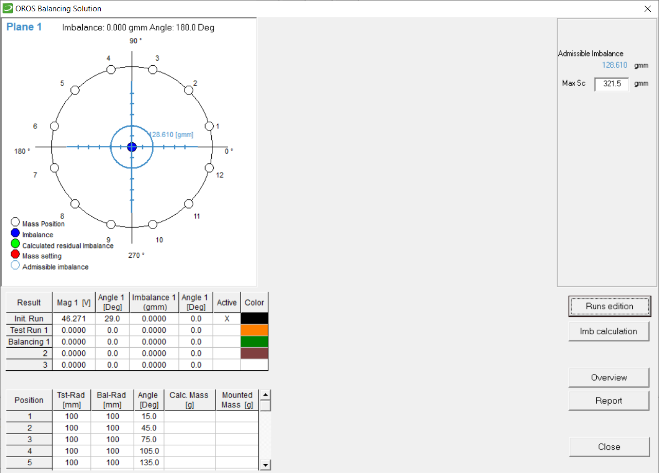
The figure below shows the result of the initial run. | The figure below shows the result of the initial run. | ||
[[Image: | [[Image:Bal_1_Init.png|framed|none]] | ||
''Initial run - start average'' | ''Initial run - start average'' | ||
| Line 406: | Line 408: | ||
Polar graph: The blue point represents the magnitude and phase of the first order of averaged order spectrum (10 averages). Click "Initial run" '''(1)''' </font>and save the initial measurement '''(2)'''</font>. | Polar graph: The blue point represents the magnitude and phase of the first order of averaged order spectrum (10 averages). Click "Initial run" '''(1)''' </font>and save the initial measurement '''(2)'''</font>. | ||
[[Image: | [[Image:Bal_1_Stopped.png|framed|none]] | ||
''Initial run'' | ''Initial run'' | ||
| Line 412: | Line 414: | ||
After saving the initial run the results are displayed as shown in '''the figure below.''' | After saving the initial run the results are displayed as shown in '''the figure below.''' | ||
[[Image: | [[Image:Bal_1_Init_Result.png|framed|none]] | ||
''Results of Initial run'' | ''Results of Initial run'' | ||
| Line 418: | Line 420: | ||
On this figure, the blue circle, representing the allowed residual unbalance, shows directly after the initial run if the machine meets the required balancing quality or not. | On this figure, the blue circle, representing the allowed residual unbalance, shows directly after the initial run if the machine meets the required balancing quality or not. | ||
''' | '''Note: '''At this point the tables only show amplitude and phase. The unbalance in <nowiki>[</nowiki>g mm<nowiki>]</nowiki> or in <nowiki>[</nowiki>oz in<nowiki>]</nowiki> can only be calculated after the rotor sensitivity is measured in the test run. Click OK to proceed to the test run. | ||
===Test run=== | ===Test run=== | ||
| Line 424: | Line 426: | ||
* Fix a test mass to the rotor. | * Fix a test mass to the rotor. | ||
* Mass, value and position must be set in the rotor geometry table. | * Mass, value and position must be as set in the rotor geometry table.<br> | ||
To see the position and mass, click "Rotor" in the Measurement monitor to open the rotor geometry window'''.''' | |||
[[Image:Bal_1_Test_Prep.png|framed|none]]<br> | |||
Your settings are shown by a red point in the polar graph. If you haven't set the test mass previously, you can do it now. | |||
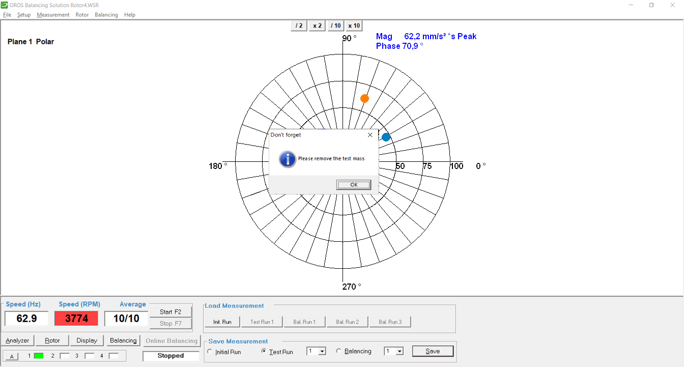
Click on OK to go back in the Measurement window. Click "Test run" '''(1)''' </font>and save the measurement '''(2)'''</font>. | |||
Click "Test run" '''(1)''' </font>and save the measurement '''(2)'''</font>. | |||
After every test run, don<nowiki>'</nowiki>t forget to remove the test mass '''(3)'''. | After every test run, don<nowiki>'</nowiki>t forget to remove the test mass '''(3)'''. | ||
[[Image: | [[Image:Bal_1_TestRun_Save.png|framed|none]] | ||
''Test run'' | ''Test run'' | ||
| Line 457: | Line 448: | ||
The amplitude scaling of the polar graph is now displayed in unbalance unit <nowiki>[</nowiki>g mm<nowiki>]</nowiki> (blue axis). | The amplitude scaling of the polar graph is now displayed in unbalance unit <nowiki>[</nowiki>g mm<nowiki>]</nowiki> (blue axis). | ||
The blue circle now represents the allowed residual unbalance in <nowiki>[</nowiki>g mm<nowiki>]</nowiki>. | The blue circle now represents the allowed residual unbalance in <nowiki>[</nowiki>g mm<nowiki>]</nowiki> according to the specified class (ISO1940/1). | ||
The result table now shows the results for initial run and test run. | The result table now shows the results for initial run and test run. | ||
| Line 465: | Line 456: | ||
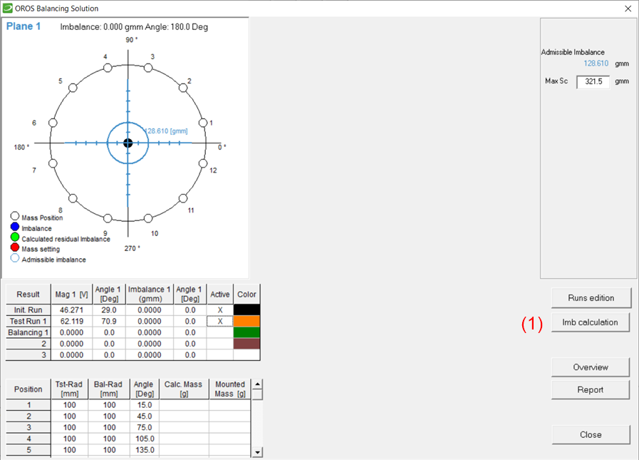
<u>Example</u> | <u>Example</u> | ||
'''(1 | '''(1)''' Click to start the calculation | ||
[[Image: | [[Image:Bal_1_test_Result.png|framed|none]] | ||
''Test run results'' | ''Test run results'' | ||
| Line 480: | Line 469: | ||
'''Orange point '''unbalance with test weight | '''Orange point '''unbalance with test weight | ||
---- | ---- | ||
| Line 489: | Line 476: | ||
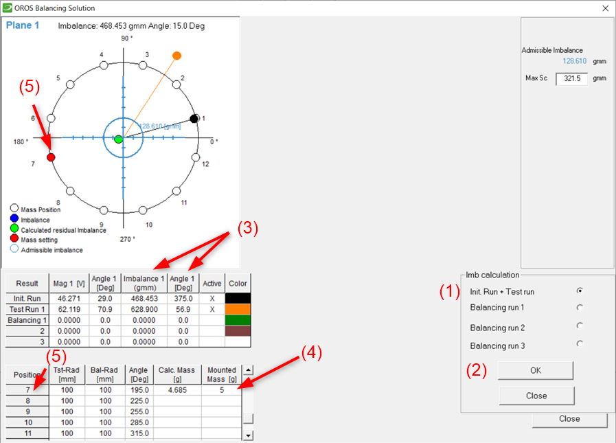
{|border="2" cellspacing="0" cellpadding="4" width="100%" | {|border="2" cellspacing="0" cellpadding="4" width="100%" | ||
|'''(1)''' </font>Select Init run <nowiki>+</nowiki> Test run<br>'''(2)''' Click OK to start the calculation<br>'''(3)''' Result - Unbalance and Phase | |'''(1)''' </font>Select Init run <nowiki>+</nowiki> Test run<br>'''(2)''' Click OK to start the calculation<br>'''(3)''' Result - Unbalance and Phase | ||
|'''(4)''' Result - proposal mass and position<br>'''(5)''' Proposal position | |'''(4)''' Result - proposal mass and position : You need to enter the real mass you will add/remove<br>'''(5)''' Proposal position | ||
|} | |} | ||
[[Image: | [[Image:Bal_1_imb_calc.png|framed|none]] | ||
''Calculation of balancing weights'' | ''Calculation of balancing weights'' | ||
If the prognostic is in the blue circle, the imbalanced of the rotor will be within the class after the mass correction. | |||
====Balancing prognosis==== | ====Balancing prognosis==== | ||
The effect of balancing weights can now be predicted by the mathematical calculations of the balancing prognosis. | The effect of balancing weights can now be predicted by the mathematical calculations of the balancing prognosis. | ||
Set mass and position of the mass you want to use in column "Mounted Mass". | Set mass and position of the mass you want to use in column "Mounted Mass". The software automatically calculates the expected residual unbalance (green point in polar graph). | ||
In this example, we only had a mass of 5 grams available instead of the calculated 4.685g mass to add at the 7th position. The prognosis shows that the residual unbalance (blue point in polar graph) moves to the green point inside the blue circle. | |||
{|border="2" cellspacing="0" cellpadding="4" width="100%" | {|border="2" cellspacing="0" cellpadding="4" width="100%" | ||
| Line 516: | Line 503: | ||
<br>Prognosis<br> | <br>Prognosis<br> | ||
| | |} | ||
====Balancing Run==== | |||
Once you have mounted the test mass as indicated by the software, you can perform a Balancing run, to ensure the rotor is now properly balanced. | |||
* Click | |||
To do so, Go back in the measurement window and press start. | |||
*'''(1)''' Click on average | |||
*'''(2)''' Select "Balancing Run1" | |||
*'''(3)''' Save the measurement | |||
| | [[Image:Bal_1_BalRun.png|framed|none]] | ||
These points only appear if they are marked "active" in the result window. Then, save the balancing result. At any stage saved results can be reloaded using the "Load Measurement" buttons. They also can be overwritten. | The orange and green point represent the initial and resulting imbalance. These points only appear if they are marked "active" in the result window. Then, save the balancing result. At any stage saved results can be reloaded using the "Load Measurement" buttons. They also can be overwritten. | ||
<u>Example</u> | <u>Example</u> | ||
| Line 535: | Line 524: | ||
'''(2)''' Click to start the calculation | '''(2)''' Click to start the calculation | ||
[[Image: | [[Image:Bal_1_BalRun_Resut.png|framed|none]] | ||
''Balancing run results'' | ''Balancing run results'' | ||
| Line 541: | Line 530: | ||
====Balancing report==== | ====Balancing report==== | ||
[[Image: | [[Image:Bal_1_Overview.png|framed|none]] | ||
''Balancing results overview'' | ''Balancing results overview''<br> | ||
The overview in the following figure now shows the chronological mass predictions and settings as well as the final result ("End"). | The overview in the following figure now shows the chronological mass predictions and settings as well as the final result ("End"). | ||
| Line 551: | Line 540: | ||
This overview can be exported into a Microsoft® Editor file (*.txt)''' '''by clicking "Report". | This overview can be exported into a Microsoft® Editor file (*.txt)''' '''by clicking "Report". | ||
[[Image: | [[Image:Bal_1_Report.png|framed|none]] | ||
''Balancing Report'' | ''Balancing Report'' | ||
| Line 560: | Line 549: | ||
===Measurements, display, storage=== | ===Measurements, display, storage=== | ||
After setting up the acquisition channel and the machine type, you may setup the test run in the "Rotor" window. For two plane balancing, you will need to perform two test run, and set a mass on each plane. By example, here, we are putting a 5g mass at pos. 3 on the first plane for the test run1 and 5g mass at pos. 8 on the second plane for the test run2. We are not putting mass on the second plane for test run1 and no mass on the first plane for test run2 : | |||
[[Image:Bal_2_TestPrep_real.png|framed|none]]<br> | |||
*'''Note :''' You may '''not''' mount the masses at this stage. <br> | |||
Then Press '''Ok''' to reach the measurement window. '''The analyser in now ready for measurement.''' | |||
'''(1)''' </font>Click "Start" start or F2. Measurement is displayed. | '''(1)''' </font>Click "Start" start or F2. Measurement is displayed. | ||
[[Image: | [[Image:Bal_2_Init.png|framed|none]] | ||
''Measurement Display'' | ''Measurement Display'' | ||
| Line 568: | Line 565: | ||
'''(1)''' </font>Click "Average" when rotor is at stable speed (Stationary state). | '''(1)''' </font>Click "Average" when rotor is at stable speed (Stationary state). | ||
[[Image: | [[Image:Bal_2_Init2.png|framed|none]] | ||
''Measurement Display'' | ''Measurement Display'' | ||
| Line 579: | Line 576: | ||
'''(2)''' Save your initial measurement | '''(2)''' Save your initial measurement | ||
[[Image: | [[Image:Bal_2_Init3.png|framed|none]] | ||
''Initial run'' | ''Initial run'' | ||
[[Image: | [[Image:Bal_2_Init_Result.png|framed|none]] | ||
''Results of Initial run'' | ''Results of Initial run'' | ||
===Test run 1 | ===Test run 1=== | ||
<u>Preparation</u> | <u>Preparation</u> | ||
| Line 601: | Line 598: | ||
* '''Keep test masses '''after test for example welding or drilling etc. | * '''Keep test masses '''after test for example welding or drilling etc. | ||
* '''Displace two masses per plane '''for machines with slidable balancing weights. | * '''Displace two masses per plane '''for machines with slidable balancing weights. | ||
It shows an example where test mass is to be removed. The test mass of | It shows an example where test mass is to be removed. The test mass of 5 grams is set at position 3 '''(1)''' </font>(75°; radius 100 mm) '''(2)''' </font> | ||
The settings are saved automatically when closing the window. | The settings are saved automatically when closing the window. | ||
[[Image: | [[Image:Bal_2_Test_PrepRun1.png|framed|none]] | ||
''Test mass positioning for two planes - Test run 1 - Test mass 1 - Plane 1'' | ''Test mass positioning for two planes - Test run 1 - Test mass 1 - Plane 1'' | ||
[[Image: | [[Image:Bal_2_TestRun1.png|framed|none]] | ||
''Test run 1'' | ''Test run 1'' | ||
| Line 617: | Line 614: | ||
After every test run, don<nowiki>'</nowiki>t forget to remove the test mass '''(3)'''. | After every test run, don<nowiki>'</nowiki>t forget to remove the test mass '''(3)'''. | ||
[[Image: | [[Image:Bal_2_TestRun1Fin.png|framed|none]] | ||
''Remove Test mass 1'' | ''Remove Test mass 1'' | ||
[[Image: | [[Image:Bal_2_TestRun1_Result.png|framed|none]] | ||
''Test run 1 results'' | ''Test run 1 results'' | ||
===Test run 2=== | |||
<u>Preparation</u> | <u>Preparation</u> | ||
| Line 638: | Line 636: | ||
* '''Keep test masses '''after test for example welding or drilling etc. | * '''Keep test masses '''after test for example welding or drilling etc. | ||
* '''Displace two masses per plane '''for machines with slidable balancing weights. | * '''Displace two masses per plane '''for machines with slidable balancing weights. | ||
An example is shown where test mass is to be removed. The test mass of 5 grams '''(4)''' </font>is set at position 8 (225°; radius 100 mm) '''(3)'''</font> | |||
The settings are saved automatically when closing the window. | The settings are saved automatically when closing the window. | ||
[[Image: | [[Image:Bal_2_Rotor_2.png|framed|none]] | ||
''Test mass 2 positioning for two planes - Test run 2 - Test mass 2 - Plane 2'' | ''Test mass 2 positioning for two planes - Test run 2 - Test mass 2 - Plane 2''<br> | ||
You can now perform the measurement of the second test run as previously ( click '''Start/F2''' and '''Average'''). Then, to save the measurement, set the Run number to 2 (1) </font>and save the measurement (2).</font> | |||
[[Image: | [[Image:Bal_2_testRun2_1.png|framed|none]] | ||
''Test run 2'' | ''Test run 2'' | ||
[[Image: | [[Image:Bal_2_TestRun2_Fin.png|framed|none]] | ||
''Remove Test mass 2'' | ''Remove Test mass 2'' | ||
| Line 660: | Line 658: | ||
'''(1)''' </font>Results for Plane 1 and Plane 2 | '''(1)''' </font>Results for Plane 1 and Plane 2 | ||
'''(2)''' | '''(2)''' Click to start the calculation | ||
[[Image: | [[Image:Bal_2_TestRun2_Result2.png|framed|none]] | ||
''Test run 2 - Result, Save and Start Calculate'' | ''Test run 2 - Result, Save and Start Calculate'' | ||
| Line 677: | Line 673: | ||
'''(2)''' Click OK to start the calculation | '''(2)''' Click OK to start the calculation | ||
[[Image: | [[Image:Bal_2_imbal_Calc.png|framed|none]] | ||
''Test run 2'' | ''Test run 2'' | ||
| Line 705: | Line 701: | ||
'''(6)''' Proposal mass and position Plane 2 | '''(6)''' Proposal mass and position Plane 2 | ||
[[Image: | [[Image:Bal_2_imbal_Calc_2.png|framed|none]] | ||
''Test run results'' | ''Test run results'' | ||
| Line 716: | Line 712: | ||
Click on "Prognosis" to get the calculation of the expected residual unbalance (green point in polar graph). | Click on "Prognosis" to get the calculation of the expected residual unbalance (green point in polar graph). | ||
Masses of 1 and 3.5 grams were available, and set to positions 5 and 6 on the first plane, and calculated masses are too small for the second plane. Therefore, we don't mount masses on the second plane as it is already balanced. <br> | |||
The prognosis shows that the residual unbalance (light green point in polar graph) moves inside the blue circle. | |||
[[Image: | [[Image:Bal_2_MountedMass.png|framed|none]] | ||
''Prognosis'' | ''Prognosis'' | ||
| Line 724: | Line 722: | ||
<u>Execution:</u> | <u>Execution:</u> | ||
* Click "balancing | * Click "Online balancing" (bottom left) | ||
* Click "Start" start or F2. Measurement is displayed. | * Click "Start" start or F2. Measurement is displayed. | ||
* Click "Average", when rotor is at stable speed .(Stationary state) | * Click "Average", when rotor is at stable speed .(Stationary state) | ||
| Line 743: | Line 741: | ||
(These points only appear if they are marked "active" in the result window) | (These points only appear if they are marked "active" in the result window) | ||
To save the balancing result, go back in the standard window by clicking on '''"Standard"''' and save as usual. | |||
[[Image: | [[Image:Bal_2_onlineBal.png|framed|none]] | ||
''Balancing run'' | ''Balancing run'' | ||
| Line 758: | Line 754: | ||
* Click "Report" in''' '''to''' '''export this table into a Microsoft® Editor file (*.txt). | * Click "Report" in''' '''to''' '''export this table into a Microsoft® Editor file (*.txt). | ||
[[Image: | [[Image:Bal_2_FinalResult.png|framed|none]] | ||
''Balancing run results'' | ''Balancing run results'' | ||
| Line 766: | Line 762: | ||
====Balancing report==== | ====Balancing report==== | ||
[[Image: | [[Image:Bal_2_Overview.png|framed|none]] | ||
''Balancing results overview'' | ''Balancing results overview'' | ||
| Line 778: | Line 774: | ||
This overview can be exported into a Microsoft® Editor file (*.txt) as a Balancing Report. | This overview can be exported into a Microsoft® Editor file (*.txt) as a Balancing Report. | ||
[[Image: | [[Image:Bal_2_Report.png|framed|none]] | ||
''Balancing Report'' | ''Balancing Report'' | ||
[[Image: | [[Image:Bal_2_Before_After.png|framed|none]] | ||
''Unbalance before [[Image:Balancing_61.png]] and after [[Image:Balancing_62.png]]balancing'' | ''Unbalance before [[Image:Balancing_61.png]] and after [[Image:Balancing_62.png]]balancing'' | ||
[[Image: | [[Image:Bal_2_Before_After_2.png|framed|none]] | ||
''Vibration measurement before [[Image:Balancing_64.png]]and after [[Image:Balancing_65.png]]balancing'' | ''Vibration measurement before [[Image:Balancing_64.png]]and after [[Image:Balancing_65.png]]balancing'' | ||
Latest revision as of 14:48, 26 June 2020
Single / Dual PLANE Balancing: User's Manual
Introduction
A rotor is a shaft rotating around its axis during service. In general, such a rotor consists of a shaft with one or more discs fitted to the axle. Such discs can be fly wheels, grinding wheels, turbine wheels, etc. The shaft is usually running in bearings allowing the rotation of the body. Depending on their rotational speed, two basic categories can be defined to classify rotors: rotors with rigid shaft, and rotors with flexible shaft.
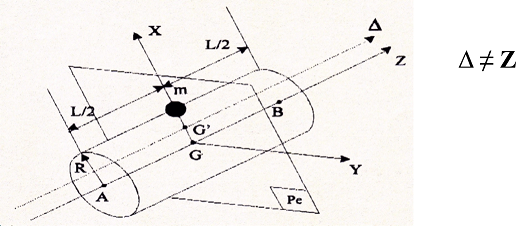
If the operating speed remains below half of the first critical bending speed, the shaft does not deflect : it may be considered as a rotor with a rigid shaft. At such operational speeds and due to the non circular cross section of the rotor, the axis of rotation (Z) and the inertial axis (Δ) does not coincide (e.g. the mass is not evenly dispatched in a section of the shaft). This may results in a tumbling movement of the structure, this amplitude depends on the bearing clearance and stiffness. In any case, the bearings are subjected to unnecessary or even not allowed loads.
At higher speeds the shaft will deflect, due to is own stiffness. In that case, it might be considered as a rotor with flexible shaft. Depending on the position of the discs on the shaft they can even be inclined and thus create an oil whirl. In that case, the Multiplane Balancing solution must be used.
An increase of the running quality is achieved through reduction of the asymmetry by means of local addition or reduction of mass. Thus the inertial axis is moved to approach the rotational axis. Rigid rotors can be sufficiently balanced in one or two planes. In practice depending of the number of transducers used and the number of planes four cases can be considered.
Case |
Number | ||
| Balancing planes | Vibration Transducers | Tach sensors | |
| 1 | 1 | 1 | 1 |
| 2 | 2 | 2 | 1 |
| 3 | 1 | 2 | 1 |
| 4 | 2 | 4 | 1 |
| Case 1 | The simplest case is to use one vibration transducer fitted for example to the rotor housing near one bearing in radial direction. | |
| Case 2 | For two planes fit one transducer near each bearing in radial direction, as above. | |
| Case 3 | To take into account the different stiffness of bearings in horizontal and vertical direction, two transducers can be used. The resultant of these two measurements is calculated and then used for balancing. To do this, transducer 1 has to be mounted radial in 45° to the horizontal, and transducer 2 in 135°. | |
| Case 4 | The same applies for two planes with 4 transducers. | |
Angular adjustments
To identify the angular position of the balancing masses, the tach point and the accelerometer direction must be taken into account.
Angular adjustments
Tach point
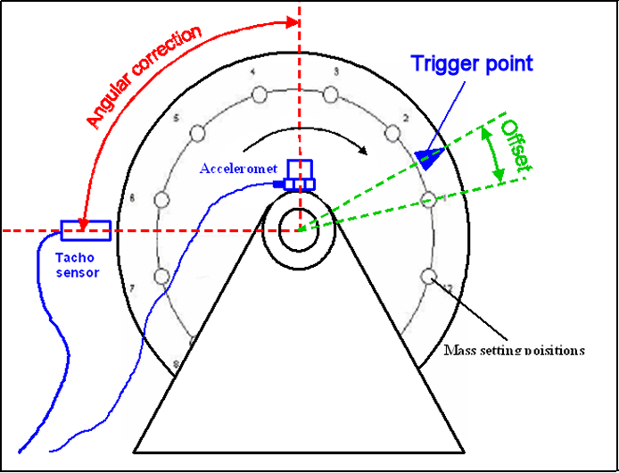
The tach trigger point should have the same angular position as position 1. If this is not possible, the angular difference can be corrected in the rotor geometry setup as "Offset".
Accelerometer
The measurement direction of the accelerometer must be referred to the tach sensor position. This can be done by the "Angular correction" in the analyzer setup. In our example, in Sketch 1, the angular correction is 90° and the offset is -15 °.
Tip
If the angular position of the tach signal is unknown, place a test mass to whatever position and define it as position 1 (0°) in the rotor geometry table. Now all angles are relative, referred to the position of the respective test mass position.
Basic balancing procedure
The execution of this balancing task can easily be achieved with your OROS 3-SERIES Analyzer (and its NVGate software running in the background) and the Balancing module. This module can be used for balancing in the lab, as well as on site. The steps in the balancing procedure are shown in the following Figures, with the corresponding explanations.
Balancing procedure
1 Initial Setting:
- Load or create a project
- Choose number of planes and Transducers (Case 1 – 4)
- Setup OROS 3-SERIES analyzer
- Introduce the rotor data
- Setup Monitor
2 Initial run
- Choose and fix a test weight
3 Test runs 1 or 2
- Calculation of the balancing weights
- Balancing prognosis
4 Balancing run
- Report
- Physical
Physical Background
The initial run analyzes the behavior of the rotor due to its initial unbalance.
During the test run, the applied test masses modify the position of the unbalance. This yields the sensitivity of the rotor. Thus with the knowledge of the reaction of the rotor to added masses, suitable masses can be calculated to compensate the initial unbalance.
For balancing in one plane, just one test mass and one test run is necessary. It is important that the angular position of the initial unbalance is changed significantly by the test mass. Take this into account when choosing test weight and position.
When balancing in two planes, two test runs are necessary. For each run only one test mass is necessary to be positioned in one of both planes respectively. Again, in both test runs the position of the unbalance must be changed by the test masses.
Assumptions
We assume a linear system. This means the rotor has to run at one stable speed during all measurement runs. The system has to be in a stationary state. If any alterations of the vibration behavior occur during the balancing procedure no meaningful balancing calculations can be obtained. Only the test weight should modify the unbalance of the rotor, but the rest of the system has to stay unchanged.
Example
Imagine a rotating machine to be balanced when standing untightened on the floor. After the test mass is mounted the increased unbalance causes the machine to move. Holding or fixing the machine during the test run will cause wrong balancing results. To overcome this you must choose a lower test mass or position to reduce the unbalance. If this doesn't work you could fix the machine during the complete balancing procedure. After this basic balancing, execute a second complete balancing procedure with the machine unfixed (in normal operating conditions).
General advice
If the test weight does not sufficiently modify the angular position of the unbalance, the rotor sensitivity can not be determined precisely, and balancing calculation is not meaningful. If the program detects this case, it will give a corresponding error message.
If no improvement is achieved during a complete balancing run, the angular position of the initial unbalance and the unbalance obtained after positioning of the test mass should be checked. If the difference is less than 10° the test run must be repeated with a different position of the test mass.
Notice: Before repeating the test run with weights in new positions, the balancing weights should be removed. After the test run balancing weights should be calculated again. Now the balancing run can be repeated.
Getting started
To start the application, click on the Balancing-Solution-Icon.
Balancing Solution
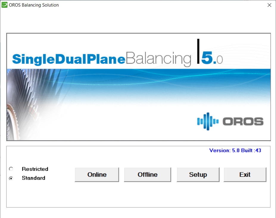
The OROS Single / Dual Balancing module appears with the following start screen
Start Balancing Solution of rigid rotors
- "Online" to start measurements, lunching NVGate.
- "Offline" to run the software offline.
- "Setup" to enter in the parameters of Balancing (selection of the language and location of NVGate.exe).
- "Standard" mode : Full access to the software
- "Restricted" mode : Restricted access (do not allow to create a new project)
When starting online the system automatically start NVGate, while displaying the dialog window below.
NVGate start request
Then, select the running mode.
Select the NVGate mode
- To proceed to a measurement, start NVGate in "Connected mode"
- For Offline access the "Office mode" can also be used.
- When the software starts, the NVGate software is displayed. Minimize NVGate.
- NVGate - Start'n Go
It is recommended to start with a default project. It is recommended to set your special user name to "Restricted user" to prevent any further changes of your settings. Then, the NVGate window can be minimized.
Settings
Settings follow the same steps whether it is for one plane balancing (single) or two planes balancing (dual). Thus, description below is given for the balancing of a two planes rotor.
Project management
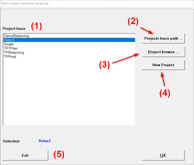
Project Manager window
| (1) Project Base : List of the project in the current Project Base (2) Projects Base Path :Change the Project Base (3) Project Browse : Add project in the current Base. |
(4) New Project : Create a new project (5) Exit : Exit the balancing program |
Load an existing Project
To load an existing project, select the project in the (1) Project Base and click OK.
You can import a project form another database by clicking on (3) Browse Project.
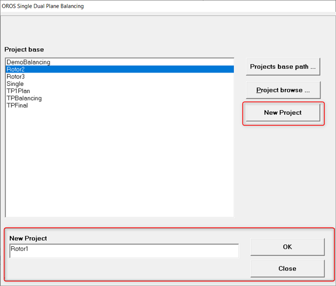
Create a new Project
To create a new project, click on (4) New Project and enter the name of the project in the appearing ribbon at the bottom of the window :
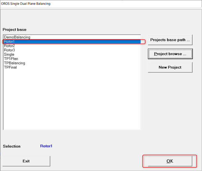
The new project will then appear in the Project Base, select it and click OK :
Select the configuration of the machine
This window, called "Analyser", will help you to quickly setting up your measurement.
First, select the configuration of your machine according to the number of planes, the geometry of the rotor (pos. of planes and bearings) and the number of vibration sensors.
Here, we are selecting a two planes rotor, with both planes between the bearings and 2 sensors.
Connect your transducers to the corresponding inputs on your 3-SERIES analyzer. The Balancing program will automatically associates the physical inputs of the frontend with the channels for the balancing according to the drawing : In1 is the channel 1 of the frontend, In2 is the channel 2, In3 the channel 3 and In4 the channel 4.
Dynamical Channels settings
Once you have selected the correct type of machine and connected the sensors to the frontend, you may go in the "Input" Tab to set your channels.
Adjustment of channels
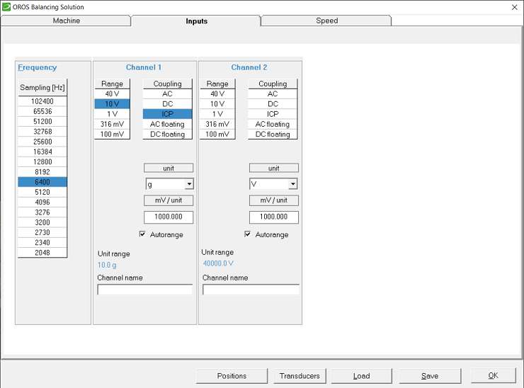
Set the input range and the coupling for your transducer, as well as his unit and sensitivity and physical quantity. You may also set the Sampling rate according to the maximal Rotating speed of the shaft (The sampling rate must be higher than the double of the max RPM*60).
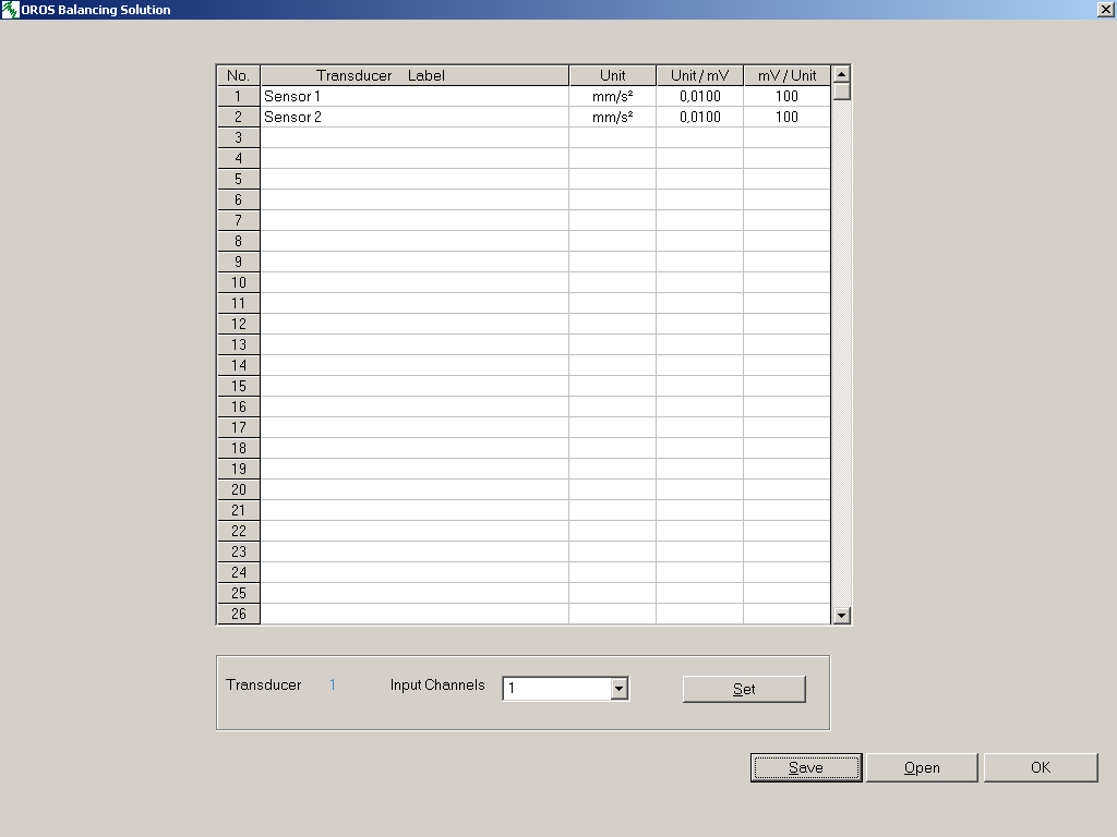
To choose your transducer from the transducer data base, click on Transducer.
Transducer database
Transducer data base
For easier and faster adjustment use the transducer data base.
Input your transducer in the list shown by clicking the corresponding fields and adjust an input transducer label, unit and sensitivity.
To select a transducer click in the corresponding line, and choose the analyzer channel, where this transducer is connected to. Click Set.
The transducer data base can be saved and reloaded.
It is also possible to create several data bases for example for different users and their transducers.
Setting the tachometer
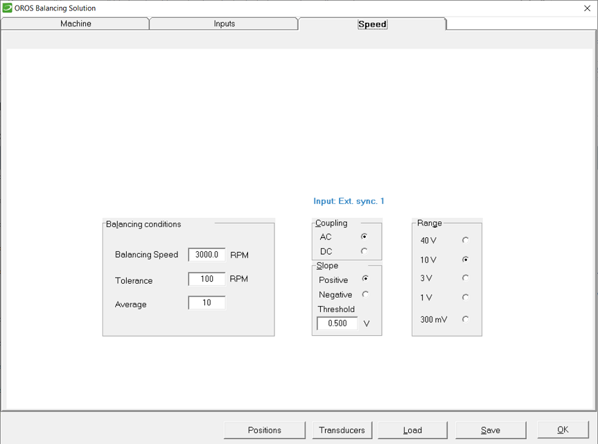
To set the tachometer, you need to go into the "Speed" tab :
Note: Your tach signal must have one pulse per revolution. If you have more than one pulse, you can set the maximal speed as Real_speed*Pulse/rev.
- Set the range, coupling and slope for this tach signal.
- Input the balancing speed.
- Set the number of averages for your measurements.
Set a phase adjustment
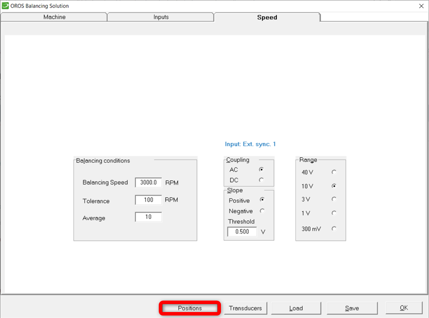
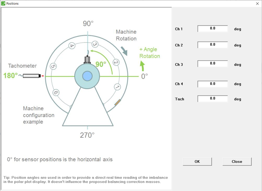
To set a phase adjustment, you can specify the position of the sensors. To enter the menu, click on "Position":
The position of each sensors and the tachometer can be set :
Note : The 0° position is the position of the tachometer reflector on the shaft. The angle are counted positive in the anti-rotation direction.
Saving the channel and measuring setup
All setup settings can be saved and reloaded with "Save" and "Load" buttons.
Note: The balancing module always starts with the last analyzer settings used.
You do not need to do all adjustments for a new project. Just load the setup of an existing project.
Tip:
If you want to make sure you always start with the same settings, create a reference project with all settings adjusted properly. Each part of the project is saved with a specific extension.
- Reference Project = *.WSR
- Analyzer settings = *.STP
- Monitor = *.DGW
- Rotor geometry = *.ROT (created when saving *.STP)
In the file menu, "File / Save Project" can be used to save the project.
For a new Project with these Settings: Load Reference Project.
This is now the last project that has been used:
- Create New Project: It has the settings of the Reference Project.
- Click "Transducer" to open the data base.
Or
- Click "Continue" to proceed to the next step.
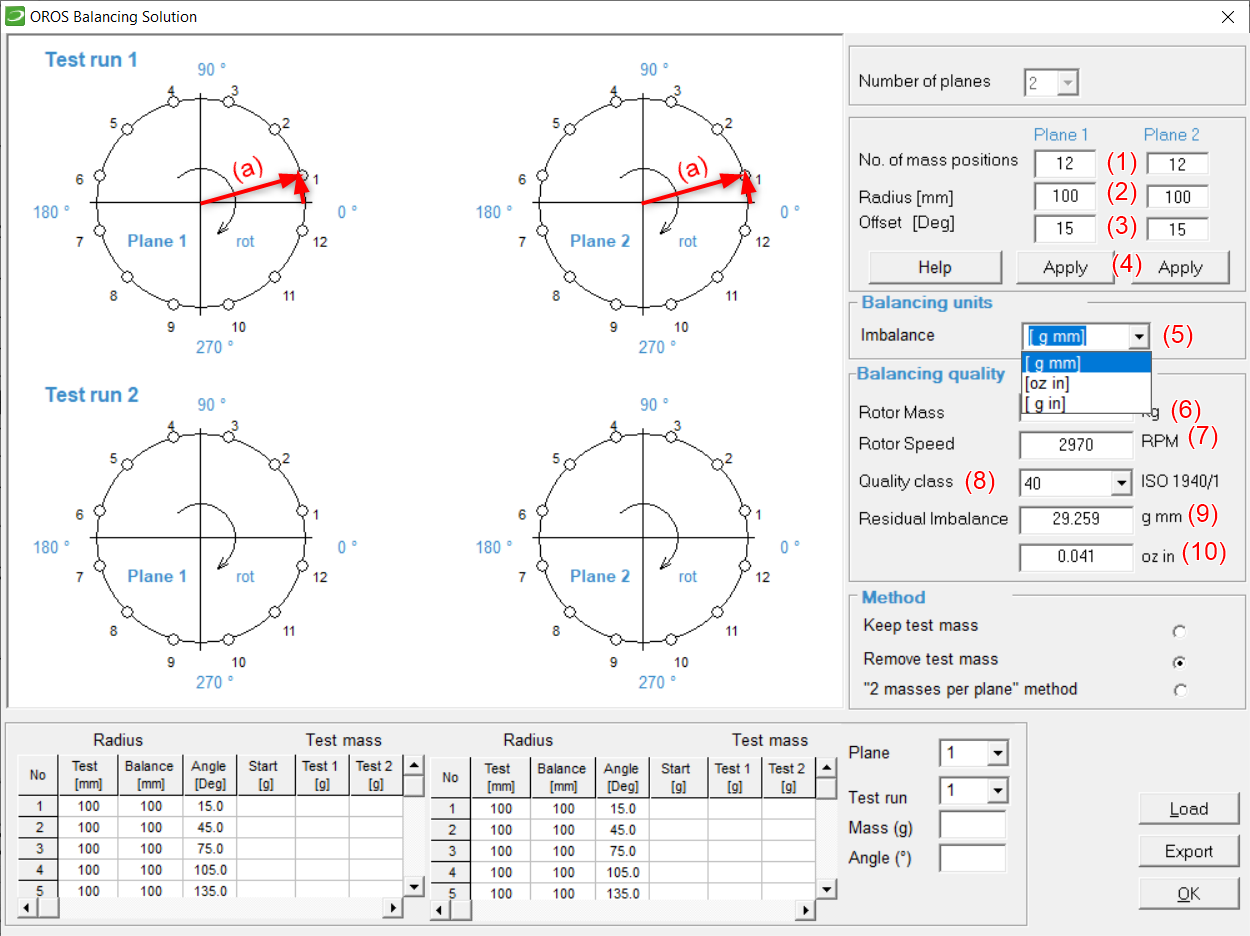
Rotor geometry and balancing quality
| (1) No. of mass positions both planes (2) Radius for both planes[mm] (3) Offset of the first mass position regarding the reference at 0° [Deg] (4) Click on Apply to display the circle (5) Unit of Unbalance [g mm], [oz in] or [g in] |
(6) Rotor mass (7) Speed RPM (8) Quality class (def. in ISO1940/1) (9) Maximal residual unbalance (according to ISO1940) [g mm] (10) Residual unbalance [oz in] |
Rotor geometry and balancing quality
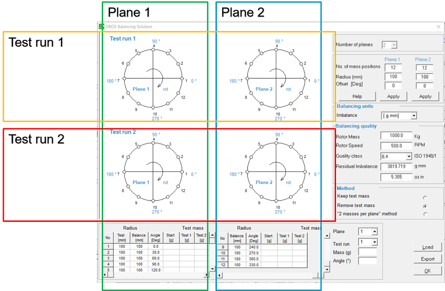
In this window, the test runs and plane are positioned as follow :
You can export and reload a configuration with the "Export" and "Load" buttons.
One plane balancing
Measurements, display, storage
Execute the following balancing procedure:
- Initial run
- Test run
- Calculation of balancing weights
- Balancing run
All runs can be saved, reloaded and overwritten.
If you use accelerometers for your measurement the signal can be integrated to show vibration velocity.
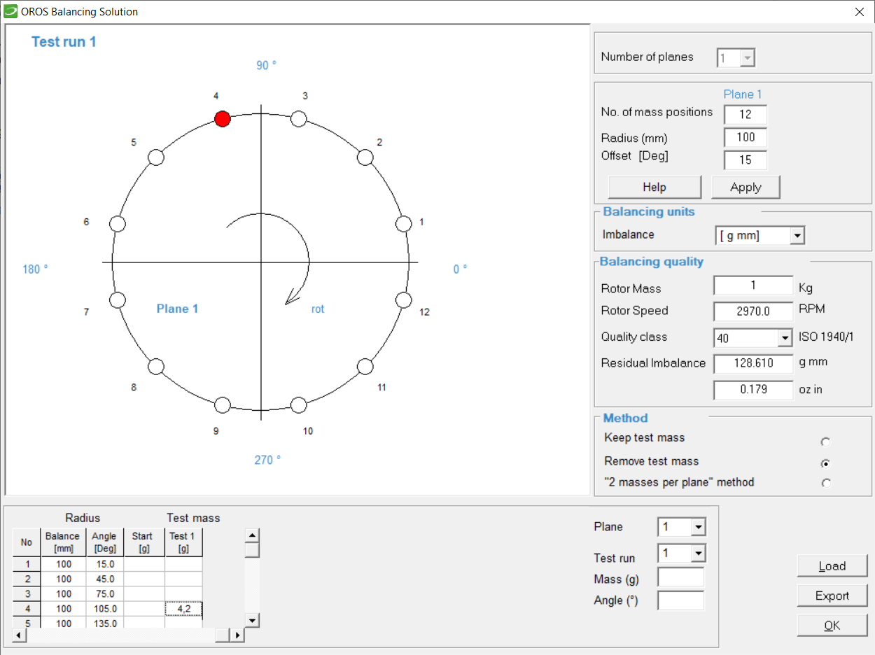
The Rotor window is automatically displayed. You can now prepare your test run or close this window to set it up later:
Your settings are shown by a red point in the polar graph.
There are three methods:
- Remove test masses : The test mass will be removed after test for example bolts etc.
- Keep test masses : The test mass cannot be removed after the test (for example for welding or drilling etc…)
- Displace two masses per plane for machines with slidable balancing weights.
The figure below shows an example where test mass is to be removed. The test mass of 4.2 grams is set at position 4 (105°; radius 100 mm).
The settings are saved automatically when closing the window. To use these settings in another project, click on export (1) and save it in the sub directory of the other project. Proper settings can be loaded from another project (2).
Click on OK to come back on the measurment window.
The analyzer is now ready for measurement.
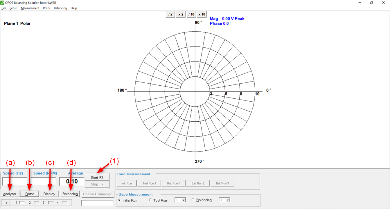
To start the analyzer click (1) or [F2] and the Measurement is displayed.
To open and changing any settings click
(a) Analyzer setup
(b) Rotor geometry and balancing quality
(c) Display setup
(d) Balancing calculation
- Measurement display - start analyzer
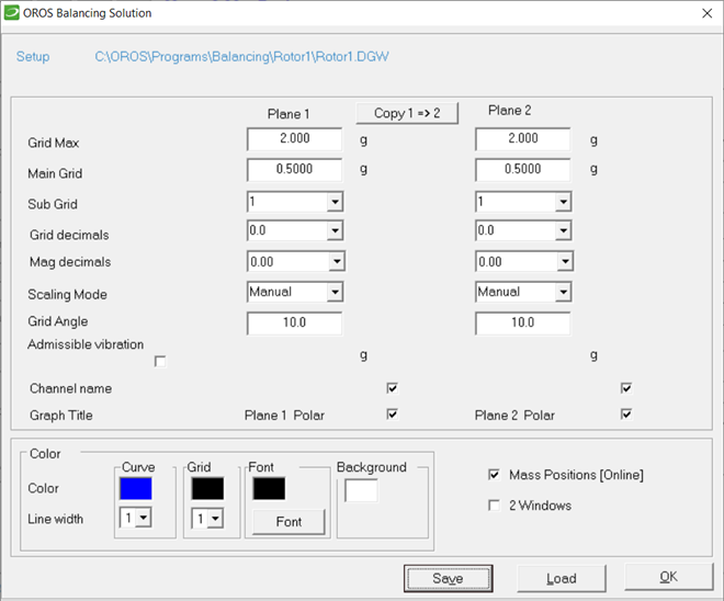
Measurement monitor settings
Display settings - Diagram 2 - Plane 2
Notice: The balancing module always starts with the monitor that has been used last.
All Settings can be modified:
- Set the number of graphs, the type and the order in which you want to see them.
Graphs with frames can be treated like windows in Windows®.
- Chose the scaling of the axis or use auto scaling (Y-axis only).
- Colors and graph names can be arranged.
- Click "Set" to create your new monitor.
- Use "Save" at the bottom to save your new monitor.
If you want to use several monitors with different layouts put existing monitors into the monitor table (double click a field in the table).
You can save and reload this selection of layouts.
Continue with "Close"
Initial run
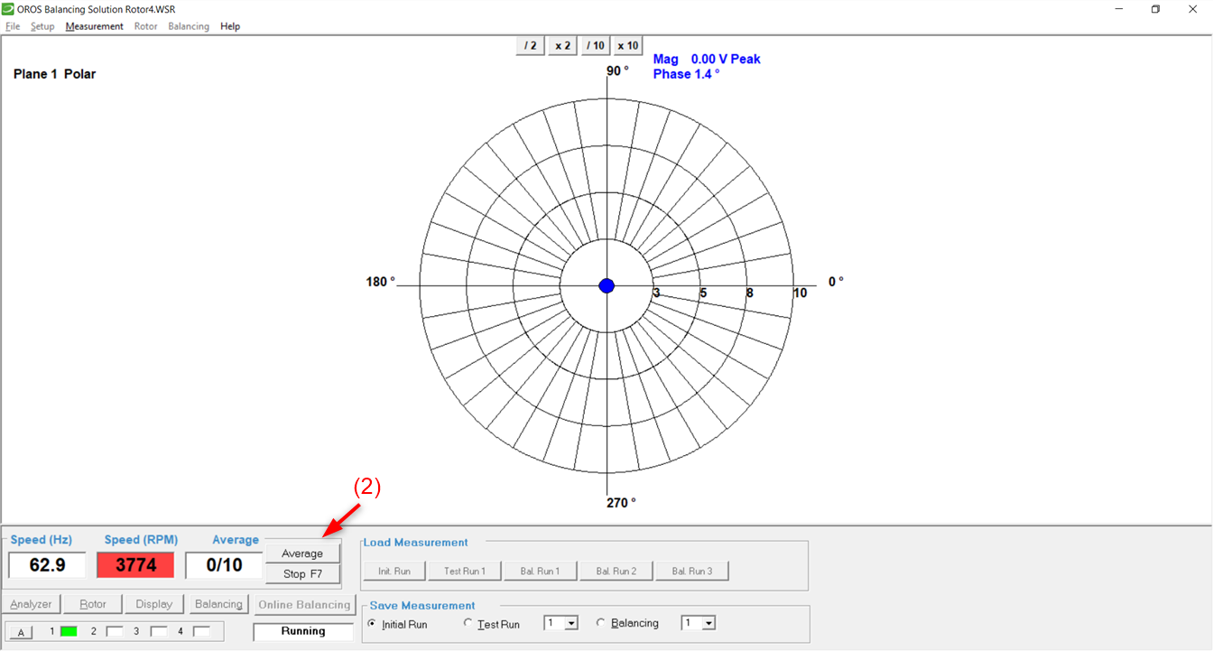
Click "Initial run"
Click "Average" (2), when rotor is at stable speed (Stationary state).
The figure below shows the result of the initial run.
Initial run - start average
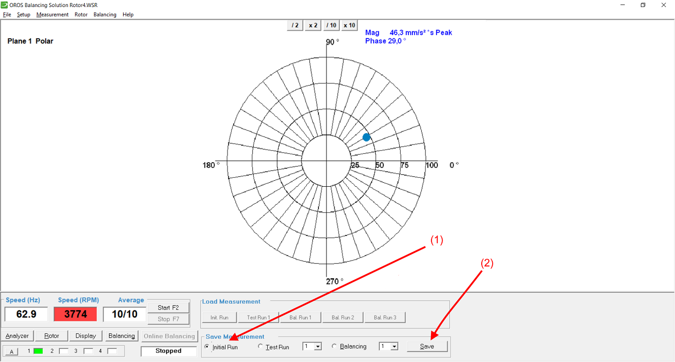
Explanation of the graphs:
Polar graph: The blue point represents the magnitude and phase of the first order of averaged order spectrum (10 averages). Click "Initial run" (1) and save the initial measurement (2).
Initial run
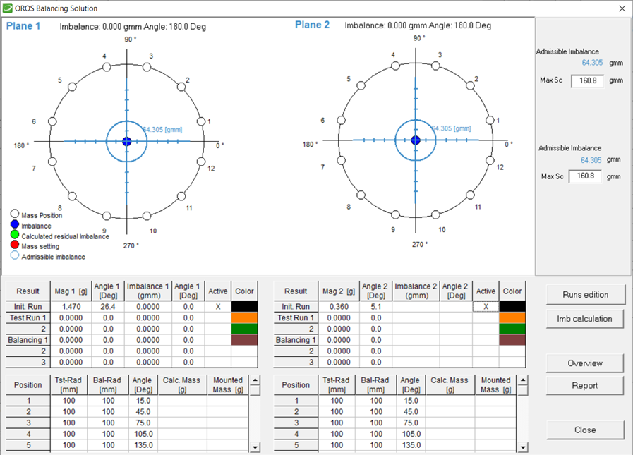
After saving the initial run the results are displayed as shown in the figure below.
Results of Initial run
On this figure, the blue circle, representing the allowed residual unbalance, shows directly after the initial run if the machine meets the required balancing quality or not.
Note: At this point the tables only show amplitude and phase. The unbalance in [g mm] or in [oz in] can only be calculated after the rotor sensitivity is measured in the test run. Click OK to proceed to the test run.
Test run
Preparation
- Fix a test mass to the rotor.
- Mass, value and position must be as set in the rotor geometry table.
To see the position and mass, click "Rotor" in the Measurement monitor to open the rotor geometry window.
Your settings are shown by a red point in the polar graph. If you haven't set the test mass previously, you can do it now.
Click on OK to go back in the Measurement window. Click "Test run" (1) and save the measurement (2).
After every test run, don't forget to remove the test mass (3).
Test run
Calculating balancing weights
After saving the test run the result is shown.
The amplitude scaling of the polar graph is now displayed in unbalance unit [g mm] (blue axis).
The blue circle now represents the allowed residual unbalance in [g mm] according to the specified class (ISO1940/1).
The result table now shows the results for initial run and test run.
Proceed to the calculation of the balancing weights now.
Example
(1) Click to start the calculation
Test run results
Click "Calculate" to determine mass and position of the balancing weights.
The weights and positions for zero unbalance appear in the table and are shown by red points.
Blue point initial unbalance
Orange point unbalance with test weight
Example
| (1) Select Init run + Test run (2) Click OK to start the calculation (3) Result - Unbalance and Phase |
(4) Result - proposal mass and position : You need to enter the real mass you will add/remove (5) Proposal position |
Calculation of balancing weights
If the prognostic is in the blue circle, the imbalanced of the rotor will be within the class after the mass correction.
Balancing prognosis
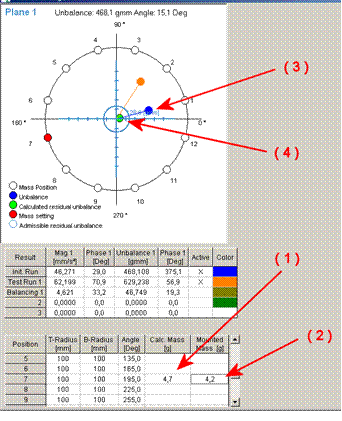
The effect of balancing weights can now be predicted by the mathematical calculations of the balancing prognosis.
Set mass and position of the mass you want to use in column "Mounted Mass". The software automatically calculates the expected residual unbalance (green point in polar graph).
In this example, we only had a mass of 5 grams available instead of the calculated 4.685g mass to add at the 7th position. The prognosis shows that the residual unbalance (blue point in polar graph) moves to the green point inside the blue circle.
| Example (1) Proposal mass and position (2) Click to enter the mass 4,2 gram (3) Initial Unbalance
(inside of the blue circle) |
|
Balancing Run
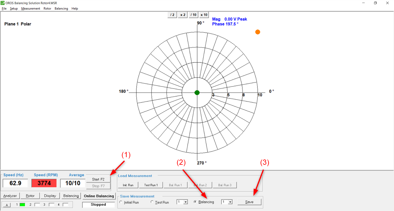
Once you have mounted the test mass as indicated by the software, you can perform a Balancing run, to ensure the rotor is now properly balanced.
To do so, Go back in the measurement window and press start.
- (1) Click on average
- (2) Select "Balancing Run1"
- (3) Save the measurement
The orange and green point represent the initial and resulting imbalance. These points only appear if they are marked "active" in the result window. Then, save the balancing result. At any stage saved results can be reloaded using the "Load Measurement" buttons. They also can be overwritten.
Example
(1) Click to save the balancing run result
(2) Click to start the calculation
Balancing run results
Balancing report
Balancing results overview
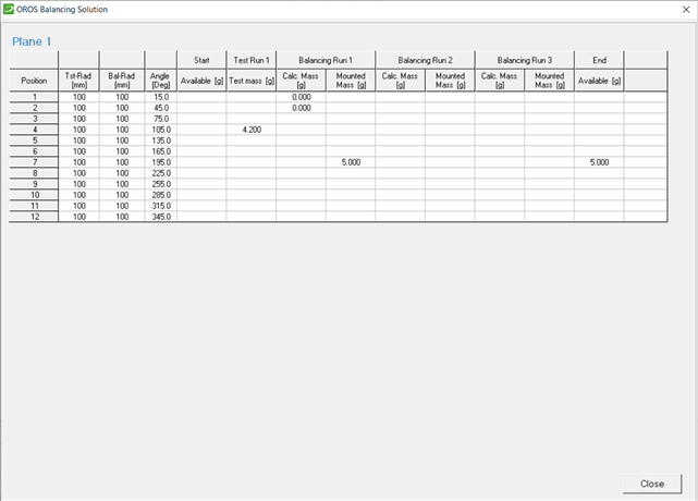
The overview in the following figure now shows the chronological mass predictions and settings as well as the final result ("End").
Also the prehistory (masses present at start of actual balancing) can be seen in column "Start".
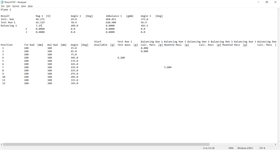
This overview can be exported into a Microsoft® Editor file (*.txt) by clicking "Report".
Balancing Report
Scroll if anything is not visible on the screen.
Two planes balancing
Measurements, display, storage
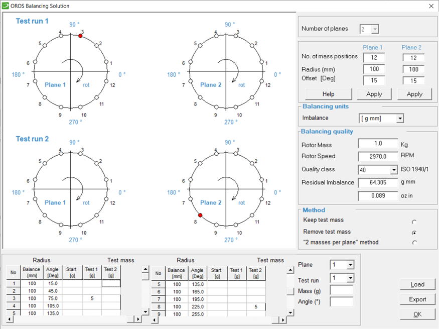
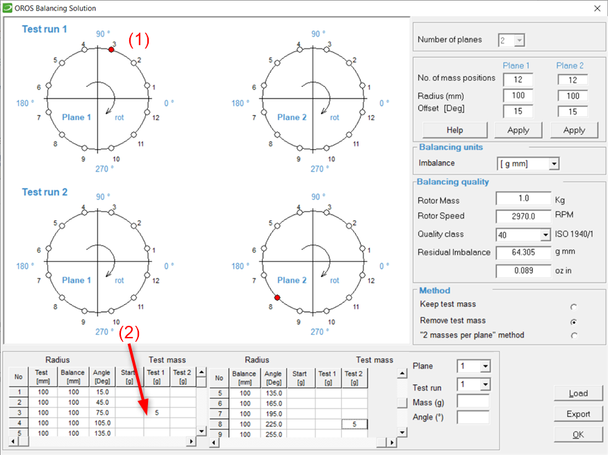
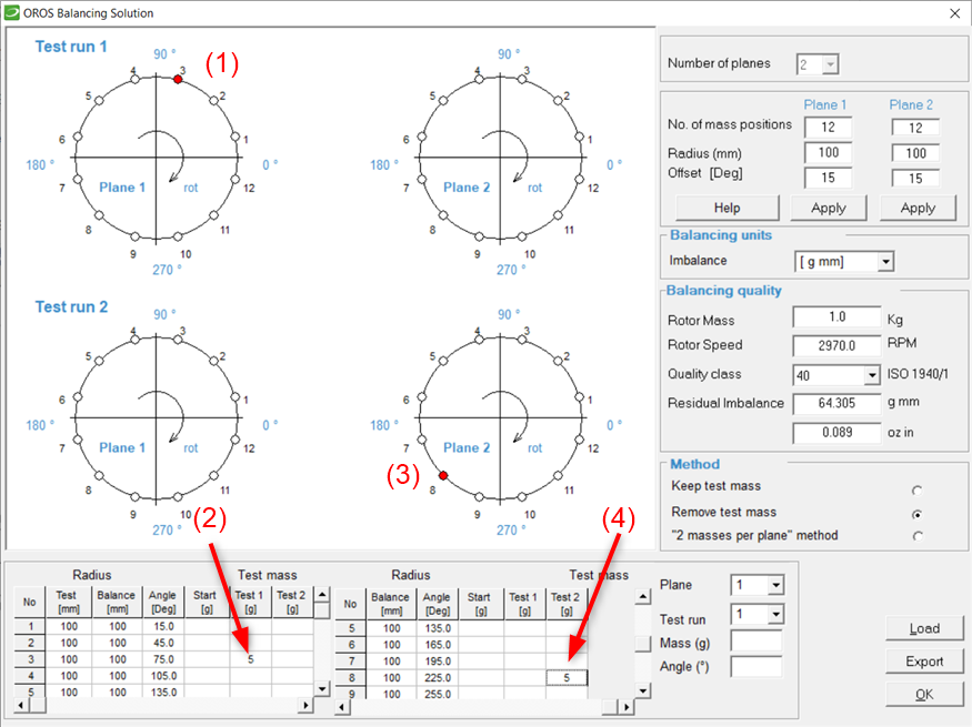
After setting up the acquisition channel and the machine type, you may setup the test run in the "Rotor" window. For two plane balancing, you will need to perform two test run, and set a mass on each plane. By example, here, we are putting a 5g mass at pos. 3 on the first plane for the test run1 and 5g mass at pos. 8 on the second plane for the test run2. We are not putting mass on the second plane for test run1 and no mass on the first plane for test run2 :
- Note : You may not mount the masses at this stage.
Then Press Ok to reach the measurement window. The analyser in now ready for measurement.
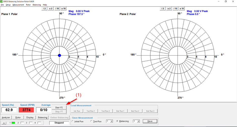
(1) Click "Start" start or F2. Measurement is displayed.
Measurement Display
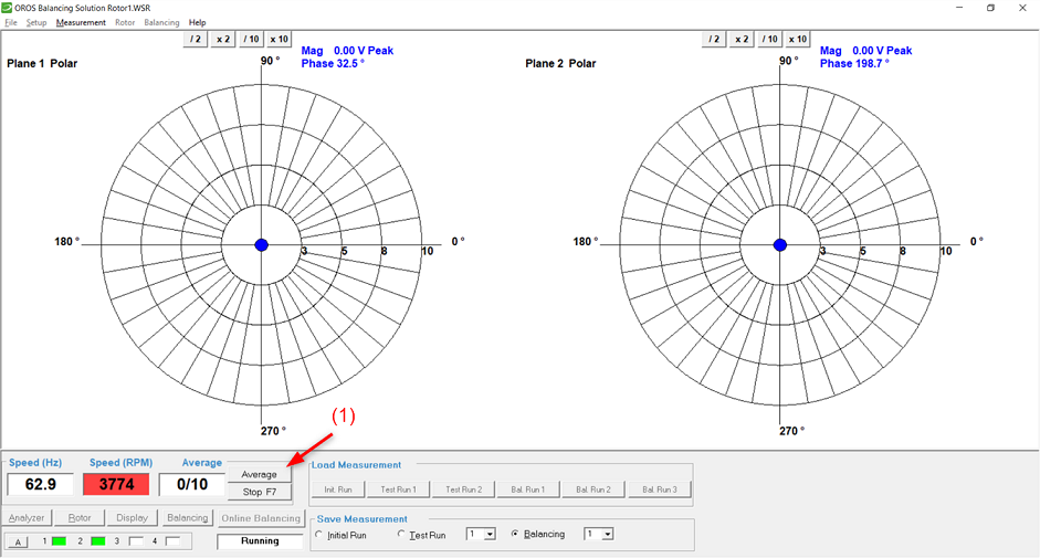
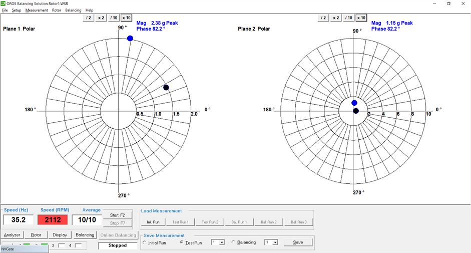
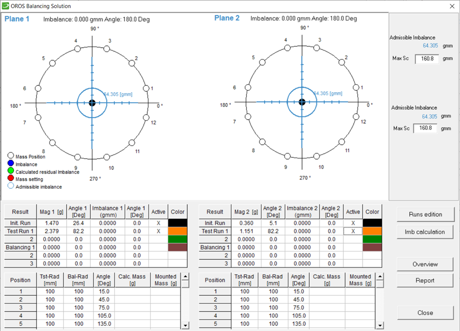
(1) Click "Average" when rotor is at stable speed (Stationary state).
Measurement Display
Initial run
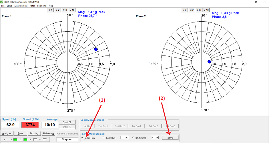
The figure shows the result of the initial run.
(1) Click "Initial run"
(2) Save your initial measurement
Initial run
Results of Initial run
Test run 1
Preparation
- Fix a test mass to the rotor.
- Mass, value and position must be set in the rotor geometry table.
To do this click "Rotor" in the Measurement monitor (b) to open the rotor geometry window.
Your settings are shown by a red point in the polar graph.
There are three methods:
- Remove test masses after test: for example bolts etc.
- Keep test masses after test for example welding or drilling etc.
- Displace two masses per plane for machines with slidable balancing weights.
It shows an example where test mass is to be removed. The test mass of 5 grams is set at position 3 (1) (75°; radius 100 mm) (2)
The settings are saved automatically when closing the window.
Test mass positioning for two planes - Test run 1 - Test mass 1 - Plane 1
Test run 1
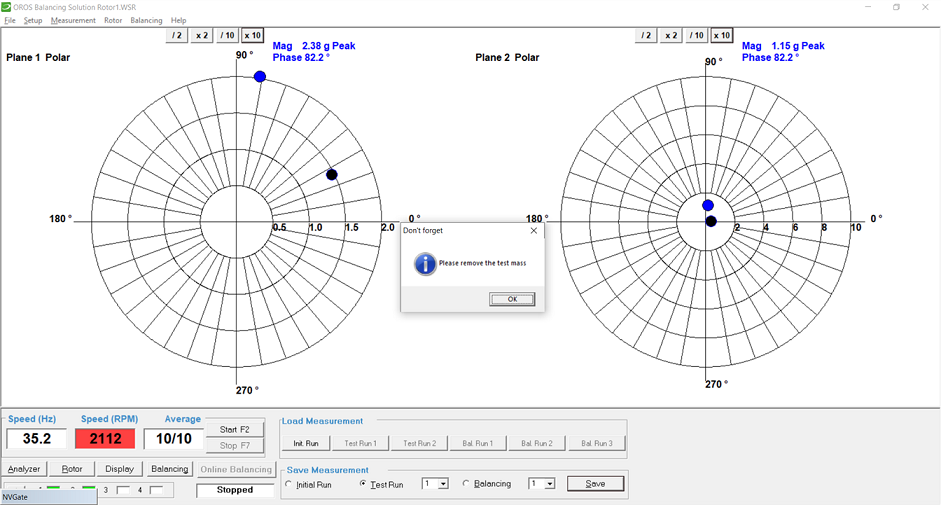
Click "Test run" (1) and save the measurement (2).
After every test run, don't forget to remove the test mass (3).
Remove Test mass 1
Test run 1 results
Test run 2
Preparation
- Fix a test mass to the rotor.
- Mass, value and position must be set in the rotor geometry table.
To do this click "Rotor" in the Measurement monitor to open the rotor geometry window.
Your settings are shown by a red point in the polar graph.
There are three methods:
- Remove test masses after test for example bolts etc.
- Keep test masses after test for example welding or drilling etc.
- Displace two masses per plane for machines with slidable balancing weights.
An example is shown where test mass is to be removed. The test mass of 5 grams (4) is set at position 8 (225°; radius 100 mm) (3)
The settings are saved automatically when closing the window.
Test mass 2 positioning for two planes - Test run 2 - Test mass 2 - Plane 2
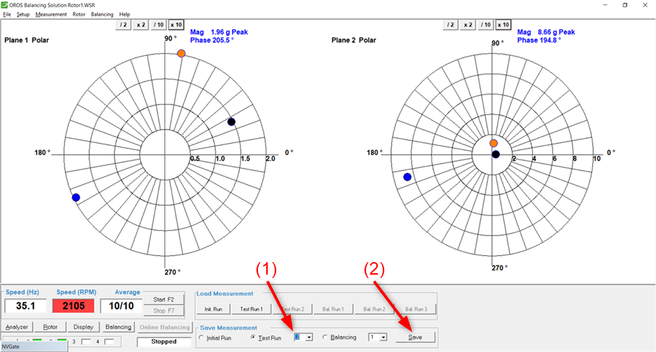
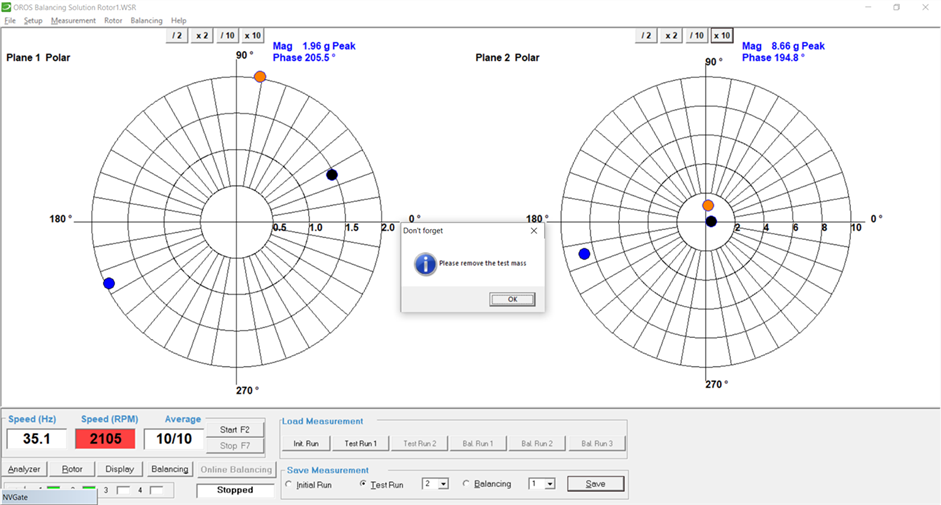
You can now perform the measurement of the second test run as previously ( click Start/F2 and Average). Then, to save the measurement, set the Run number to 2 (1) and save the measurement (2).
Test run 2
Remove Test mass 2
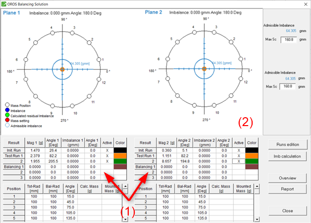
Example
(1) Results for Plane 1 and Plane 2
(2) Click to start the calculation
Test run 2 - Result, Save and Start Calculate
Calculating balancing weights
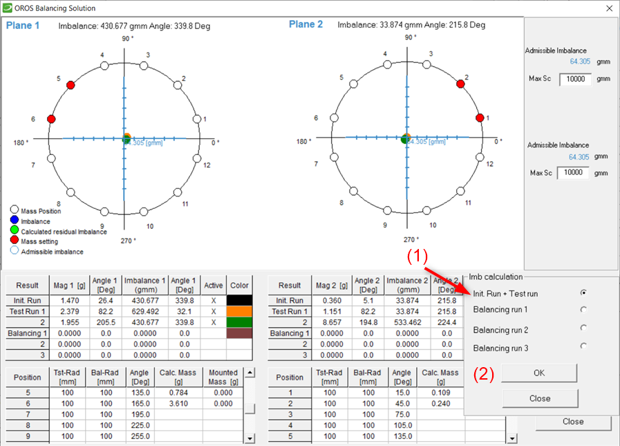
Example
(1) Select Init run + Test run
(2) Click OK to start the calculation
Test run 2
After saving the test run the result is shown.
The amplitude scaling of the polar graph is now displayed in unbalance unit [g mm] (blue axis).
The blue circle now represents the allowed residual unbalance in [g mm].
The result table now shows the results for initial run and test run.
Proceed to the calculation of the balancing weights now.
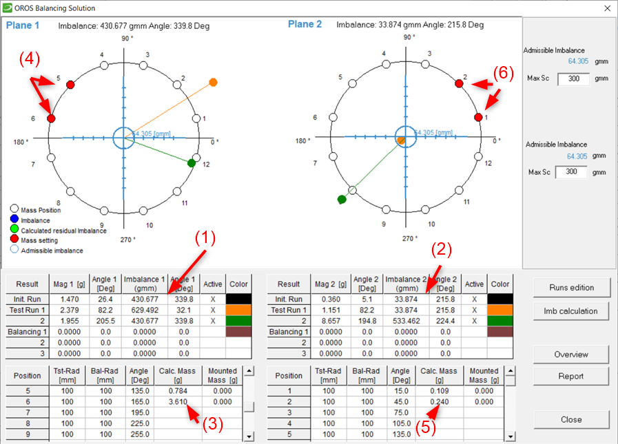
Example
(1) Result - Unbalance 1 and Phase 1
(2) Result - Unbalance 2 and Phase 2
(3) Unbalance and Phase Plane 1
(4) Proposal mass and position Plane 1
(5) Unbalance and Phase Plane 2
(6) Proposal mass and position Plane 2
Test run results
Balancing prognosis
The effect of balancing weights can now be predicted by the mathematical calculations of the balancing prognosis.
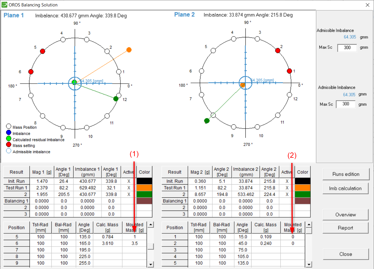
Set mass and position of the mass you want to use in column "Mounted Mass" (1), (2)
Click on "Prognosis" to get the calculation of the expected residual unbalance (green point in polar graph).
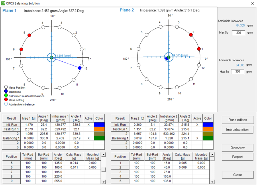
Masses of 1 and 3.5 grams were available, and set to positions 5 and 6 on the first plane, and calculated masses are too small for the second plane. Therefore, we don't mount masses on the second plane as it is already balanced.
The prognosis shows that the residual unbalance (light green point in polar graph) moves inside the blue circle.
Prognosis
Execution:
- Click "Online balancing" (bottom left)
- Click "Start" start or F2. Measurement is displayed.
- Click "Average", when rotor is at stable speed .(Stationary state)
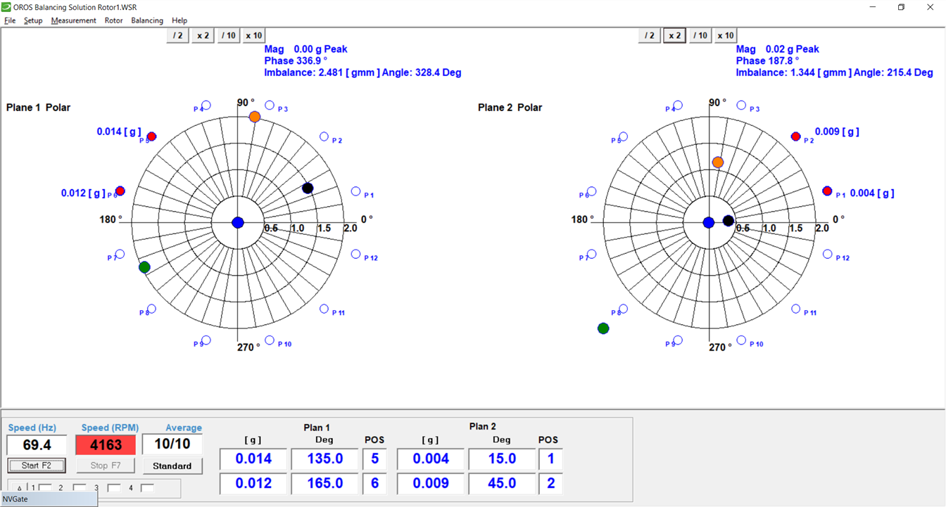
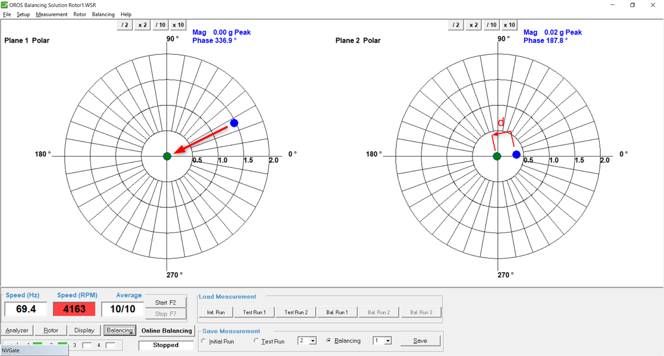
The figure below shows the result of the balancing run.
Explanation of graphs:
Polar graph;
Blue point Initial run
Orange point Test run 1
Olive point Test run 2
Green point Balancing run
(These points only appear if they are marked "active" in the result window)
To save the balancing result, go back in the standard window by clicking on "Standard" and save as usual.
Balancing run
To visualize hidden points deactivate the respective covering points. (click the respective field in column "Active" of the tables!)
The dark green point in plane 1 and the orange point in plane 2 were deactivated and the black points are visible again.
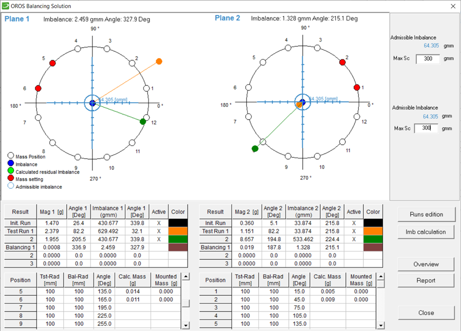
- Click "Overview" to see a summary of the whole balancing job.
- Click "Report" in to export this table into a Microsoft® Editor file (*.txt).
Balancing run results
Balancing report
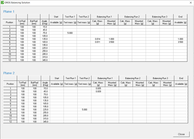
Balancing results overview
The overview now shows the chronological mass predictions and settings as well as the final result ("End").
Also the prehistory (masses present at start of actual balancing) can be seen in column "Start".
Scroll if anything is not visible on the screen.
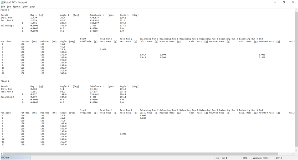
This overview can be exported into a Microsoft® Editor file (*.txt) as a Balancing Report.
Balancing Report
